In March 2021, Azure Communication Services was made generally available after being showcased in Microsoft Ignite. In the beginning, it only provides services such as SMS as well as voice and video calling. One year after that, in May 2022, it also offers a way to facilitate high volume transactional emails. However, currently this email function is still in public preview. Hence, the email relevant APIs and SDKs are provided without a SLA, which is thus not recommended for production workloads.
Currently, our Azure account has a set of limitation on the number of email messages that we can send. For all the developers, email sending is limited to 10 emails per minute, 25 emails in an hour, and 100 emails in day.
Setup Azure Communication Services
To begin, we need to createa a new Email Communication Services resource from the marketplace, as shown in the screenshot below.
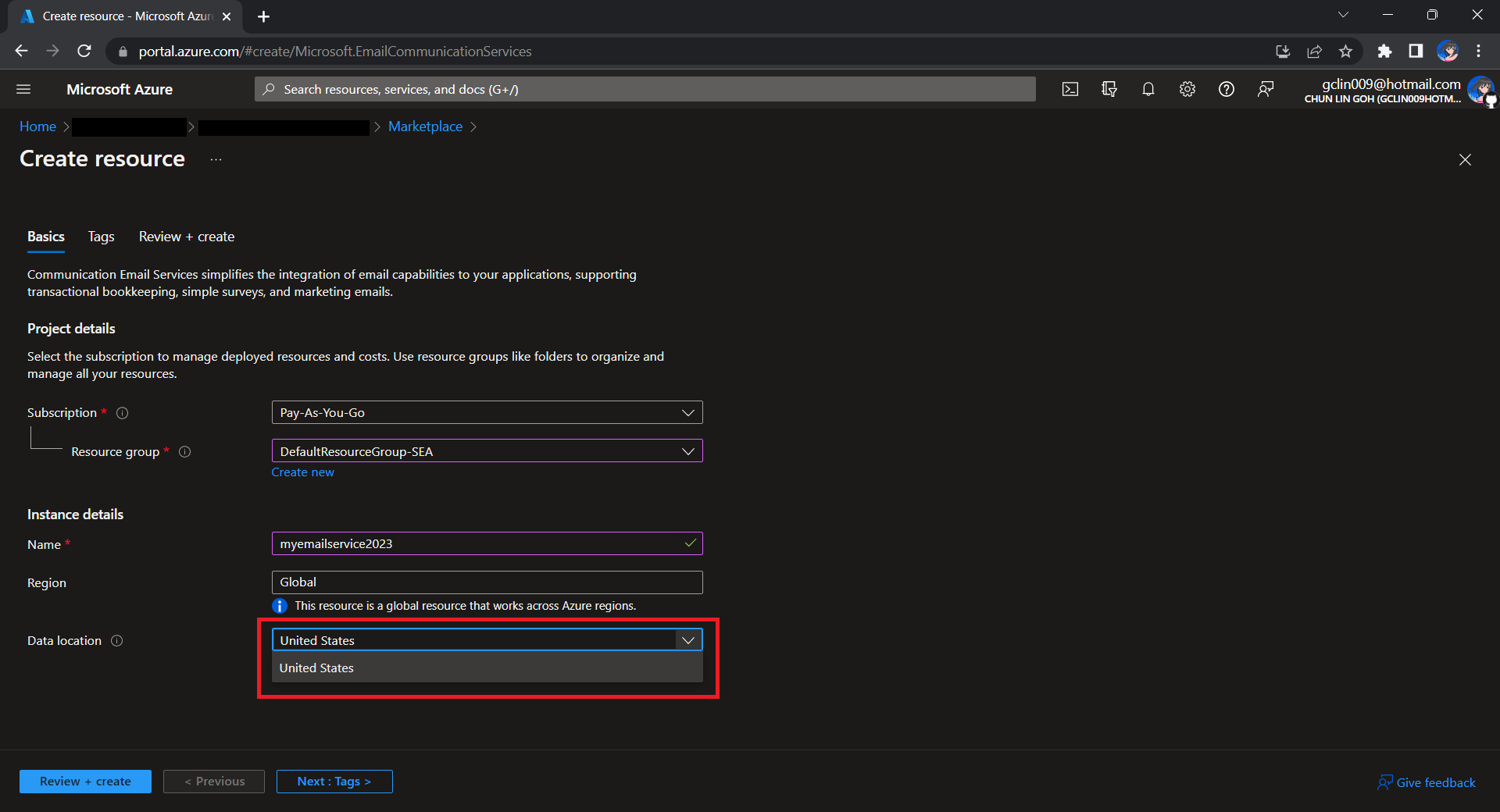
Take note that currently we can only choose United States as the Data Location, which determines where the data will be stored at rest. This cannot be changed after the resource has been created. This thus make our Azure Communication Services which we need to configure next to store the data in United States as well. We will talk about this later.
Once the Email Communication Service is created, we can begin by adding a free Azure subdomain. With the “1-click add” function, as shown in the following screenshot, Azure will automatically configures the required email authentication protocols based on the email authentication best practices.
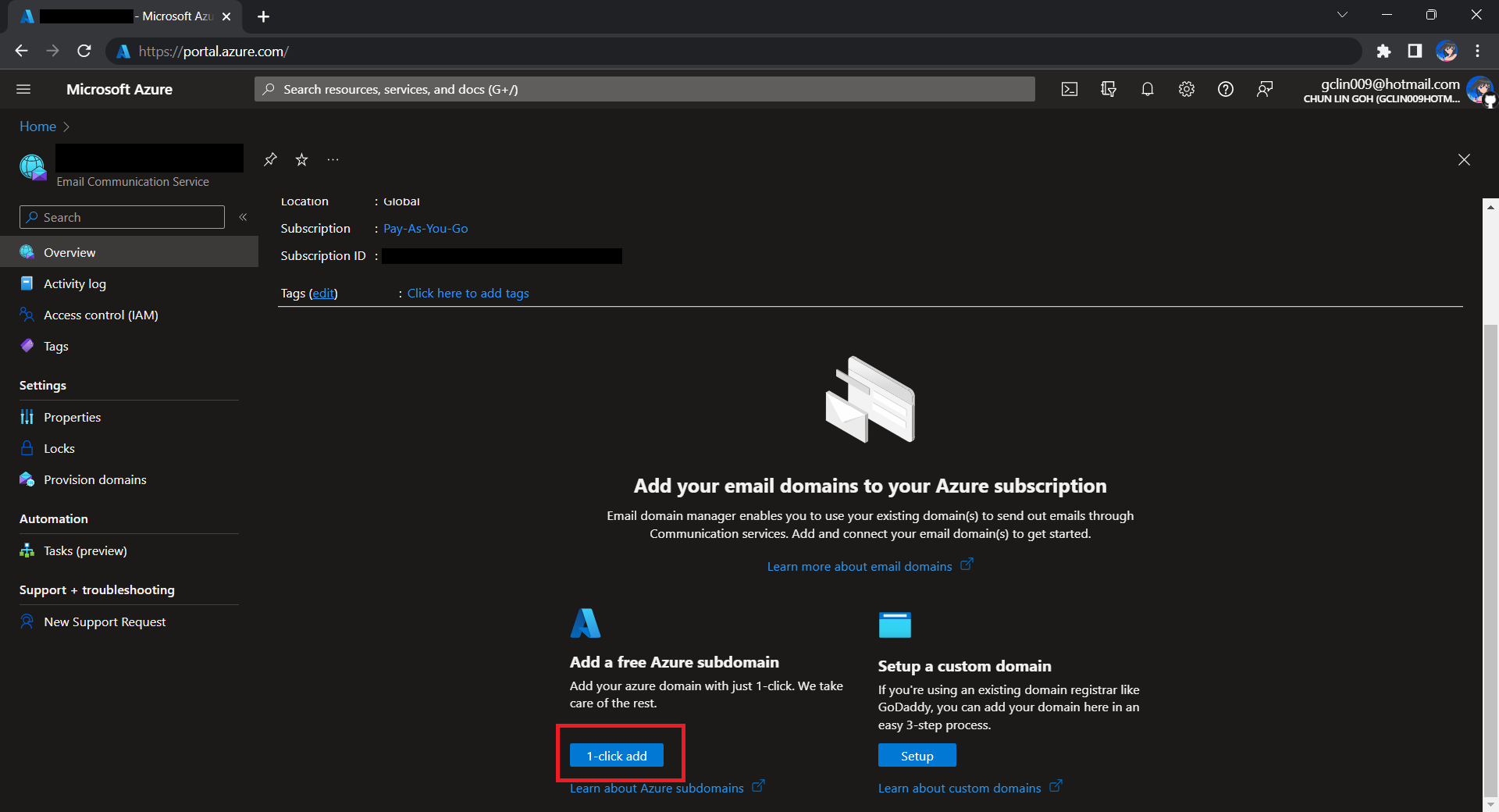
We will then have a MailFrom address in the format of donotreply@xxxx.azurecomm.net which we can use to send email. We are allowed to modify the MailFrom address and From display name to more user-friendly values.
After getting the domain, we need to connect Azure Communication Services to it to send emails.
As we talked earlier, we need to make sure that the Azure Communication Services to have United States as its Data Location as well. Otherwise, we will not be able to link the email domain for email sending.

A Simple Console App for Sending Email
Now, we need to create the console app which we will be used in our Kubernetes CronJob later to send the emails with the Azure Communication Services Email client library.
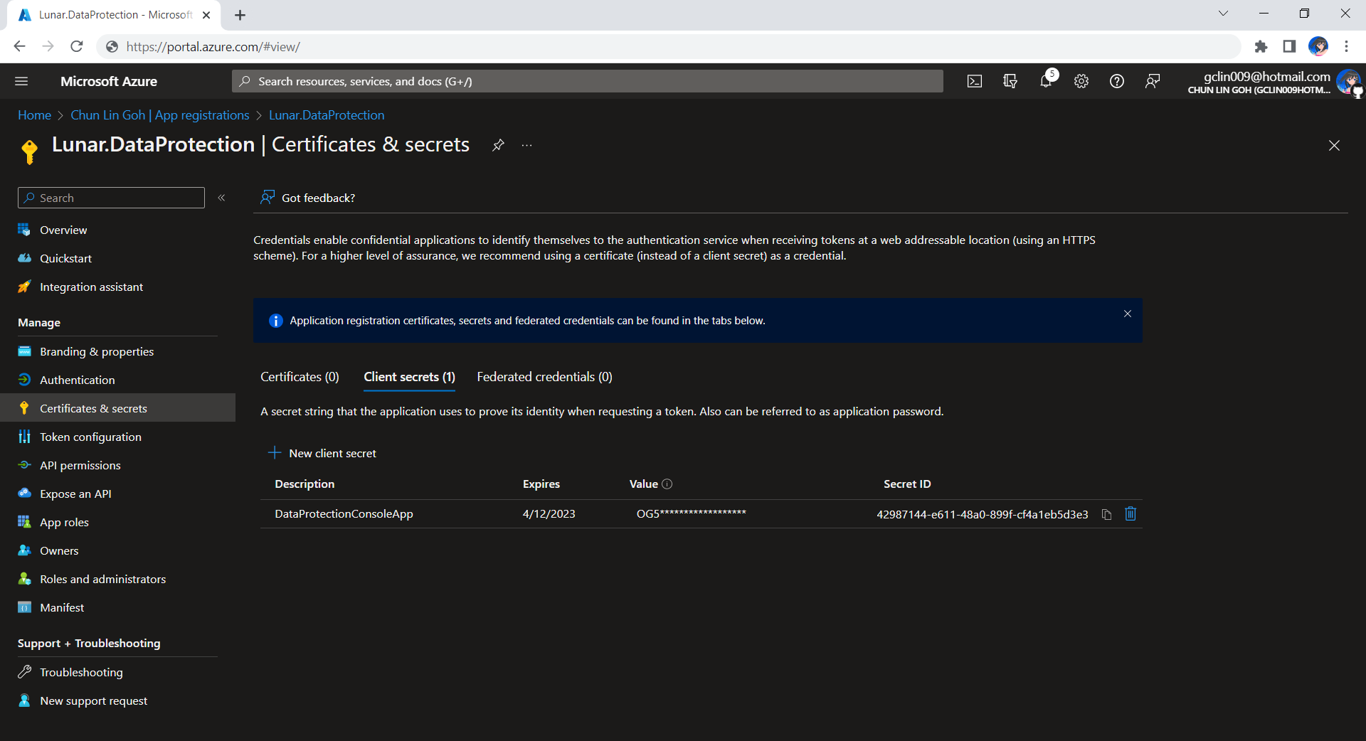
Before we begin, we have to get the connection string for the Azure Communication Service resource.
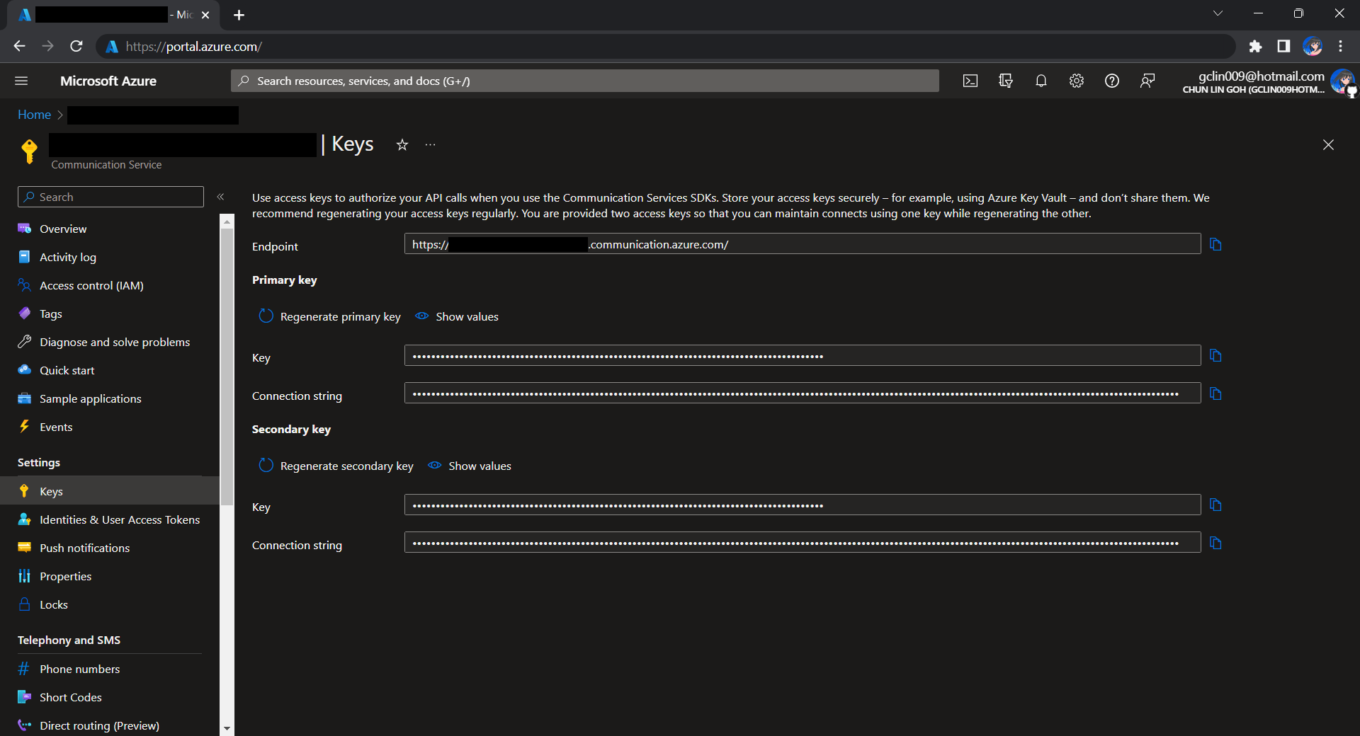
Here I have the following code to send a sample email to myself.
using Azure.Communication.Email.Models;
using Azure.Communication.Email;
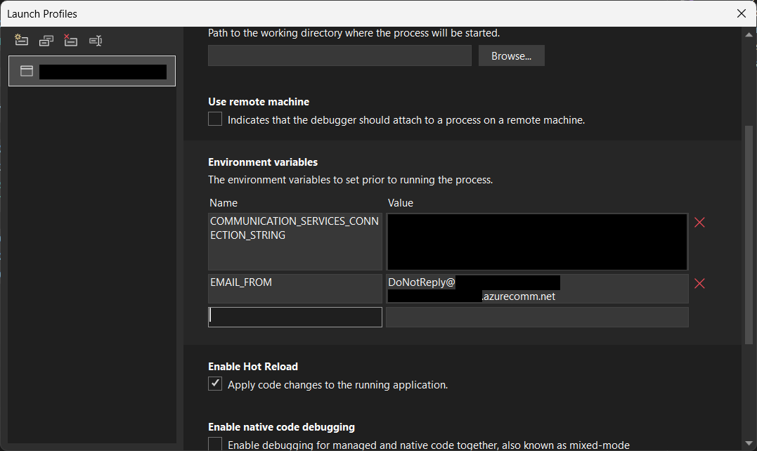
string connectionString = Environment.GetEnvironmentVariable("COMMUNICATION_SERVICES_CONNECTION_STRING") ?? string.Empty;
string emailFrom = Environment.GetEnvironmentVariable("EMAIL_FROM") ?? string.Empty;
if (connectionString != string.Empty)
{
EmailClient emailClient = new EmailClient(connectionString);
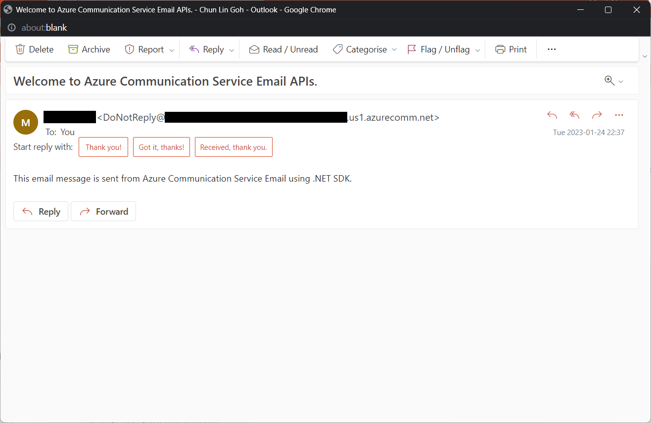
EmailContent emailContent = new EmailContent("Welcome to Azure Communication Service Email APIs.");
emailContent.PlainText = "This email message is sent from Azure Communication Service Email using .NET SDK.";
List<EmailAddress> emailAddresses = new List<EmailAddress> {
new EmailAddress("gclin009@hotmail.com") { DisplayName = "Goh Chun Lin" }
};
EmailRecipients emailRecipients = new EmailRecipients(emailAddresses);
EmailMessage emailMessage = new EmailMessage(emailFrom, emailContent, emailRecipients);
SendEmailResult emailResult = emailClient.Send(emailMessage, CancellationToken.None);
}
Tada, there should be an email successfully sent out as instructed.
Containerise the Console App
Next what we need to do is containerising our console app above.
Assume that our console app is called MyConsoleApp, then we will prepare a Dockerfile as follows.
FROM mcr.microsoft.com/dotnet/runtime:6.0 AS base
WORKDIR /app

FROM mcr.microsoft.com/dotnet/sdk:6.0 AS build
WORKDIR /src
COPY ["MyMedicalEmailSending.csproj", "."]
RUN dotnet restore "./MyConsoleApp.csproj"
COPY . .
WORKDIR "/src/."
RUN dotnet build "MyConsoleApp.csproj" -c Release -o /app/build

FROM build AS publish
RUN dotnet publish "MyConsoleApp.csproj" -c Release -o /app/publish /p:UseAppHost=false

FROM base AS final
WORKDIR /app
COPY --from=publish /app/publish .
ENTRYPOINT ["dotnet", "MyConsoleApp.dll"]
We then can publish it to Docker Hub for consumption later.
If you prefer to use Azure Container Registry, you can refer to the documentation on how to do it on Microsoft Learn.
Create the CronJob
In Kubernetes, pods are the smallest deployable units of computing we can create and manage. A pod can have one or more relevant containers, with shared storage and network resources. Here, we will be scheduling a job so that it creates pods containing our container with the image we created above to operate the execution of the pods, which is in our case, to send emails.
The schedule of the cronjob is defined as follows, according to the Kubernetes documentation on the schedule syntax.
# ┌───────────── minute (0 - 59)
# │ ┌───────────── hour (0 - 23)
# │ │ ┌───────────── day of the month (1 - 31)
# │ │ │ ┌───────────── month (1 - 12)
# │ │ │ │ ┌───────────── day of the week (sun, mon, tue, wed, thu, fri, sat)
# │ │ │ │ │
# * * * * *
Hence, if we would like to have the email scheduler to be triggered at 8am of every Friday, we can create a CronJob in the namespace my-namespace with the following YAML file.
apiVersion: batch/v1
kind: CronJob
metadata:
  name: email-scheduler
  namespace: ns-mymedical
spec:
  jobTemplate:
    metadata:
      name: email-scheduler
    spec:
      template:
        spec:
          containers:
          - image: chunlindocker/emailsender:v2023-01-25-1600
            name: email-scheduler
          restartPolicy: OnFailure
  schedule: 0 8 * * fri
After the CronJob is created, we can proceed to annotate it with the command below.
kubectl annotate cj email-scheduler jobtype=scheduler frequency=weekly
This helps us to query the cron jobs with jsonpath easily in the future. For example, we can list all cronjobs which are scheduled weekly, we can do it with the following command.
kubectl get cj -A -o=jsonpath="{range .items[?(@.metadata.annotations.jobtype)]}{.metadata.namespace},{.metadata.name},{.metadata.annotations.jobtype},{.metadata.annotations.frequency}{'\n'}{end}"
Create ConfigMap
In our email sending programme, we have two environment variables. Hence, we can create ConfigMap to store the data as key-value pair.
apiVersion: v1
kind: ConfigMap
metadata:
  name: email-sending
  namespace: my-namespace
data:
  EMAIL_FROM: DoNotReply@xxxxxx.azurecomm.net
For connection string of Azure Communication Service, since it is a sensitive data, we will store it in Secret. Secrets are similar to ConfigMaps but are specifically intended to hold confidential data. We will create a Secret with the command below.
kubectl create secret generic azure-communication-service --from-literal=CONNECTION_STRING=xxxxxx --dry-run=client --namespace=my-namespace -o yaml
It should generate a YAML which is similar to the following.
apiVersion: v1
kind: Secret
metadata:
  name: azure-communication-service
  namespace: my-namespace
data:
  CONNECTION_STRING: yyyyyyyyyy
Then, the Pods created by the CronJob can thus consume the ConfigMap and Secret above as environment variables. So, we need to update the CronJob YAML file to be as follows.
apiVersion: batch/v1
kind: CronJob
metadata:
  name: email-scheduler
  namespace: my-namespace
spec:
  jobTemplate:
    metadata:
      name: email-scheduler
    spec:
      template:
        spec:
          containers:
          - image: chunlindocker/emailsender:v2023-01-25-1600
            name: email-scheduler
            env:
              - name: EMAIL_FROM
                valueFrom:
                  configMapKeyRef:
                    name: email-sending
                    key: EMAIL_FROM
              - name: COMMUNICATION_SERVICES_CONNECTION_STRING
                valueFrom:
                  secretKeyRef:
                    name: azure-communication-service
                    key: CONNECTION_STRING
          restartPolicy: OnFailure
  schedule: 0 8 * * fri
Using SealedSecret
Problem with using Secrets is that we can’t really commit them to our code repository because the data are only encoded but not encrypted. Hence, in order to store our Secrets safely, we need to use SealedSecret which helps us to encrypt our Secret. The SealedSecret can only be decrypted by the controller running in the targer cluster.
Currently, the SealedSecret Helm Chart is officially supported and hosted on GitHub.
Helm is the package manager for Kubernetes. Helm uses a packaging format called Chart, a collection of files describing a related set of Kubernetes resource. Each Chart comprises one or more Kubernetes manifests. With Chart, developers are able to configure, package, version, and share the apps with their dependencies and sensible defaults.
To install Helm on Windows 11 machine, we can execute the following commands in Ubuntu on Windows console.
- Download desired version of Helm release, for example, to download version 3.11.0:
wget https://get.helm.sh/helm-v3.11.0-linux-amd64.tar.gz - Unpack it:
tar -zxvf helm-v3.2.0-linux-amd64.tar.gz - Move the Helm binary to desired location:
sudo mv linux-amd64/helm /usr/local/bin/helm
Once we have successfully downloaded Helm and have it ready, we can add a Chart repository. In our case, we need to add the repo of SealedSecret Helm Chart.
helm repo add sealed-secrets https://bitnami-labs.github.io/sealed-secrets
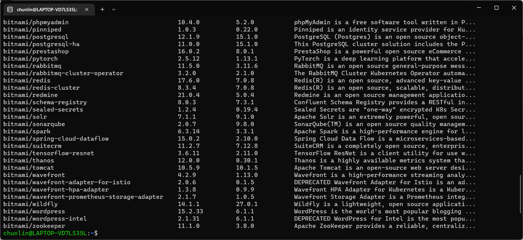
We should be able to locate the SealedSecret chart that we can install with the following command.
helm search repo bitnami
To installed SealedSecret Helm Chart, we will use the following command.
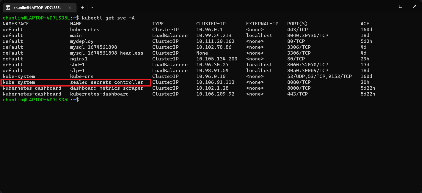
helm install sealed-secrets -n kube-system --set-string fullnameOverride=sealed-secrets-controller sealed-secrets/sealed-secrets
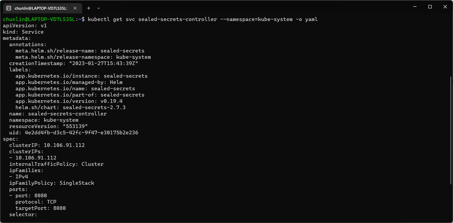
Once we have done this, we should be able to locate a new service called sealed-secret-controller under Kubernetes services.
Before we can proceed to use kubeseal to create an encrypted secret, for me at least, there is a need to edit the sealed-secret-controller service. Otherwise, there will be an error message saying “cannot fetch certificate: no endpoints available for service”. If you also encounter the same issue, simply follow the steps mentioned by ghostsquad to edit the service YAML accordingly.
Next, we then can proceed to encrypt our secret, as instructed on the SealedSecret GitHub readme.
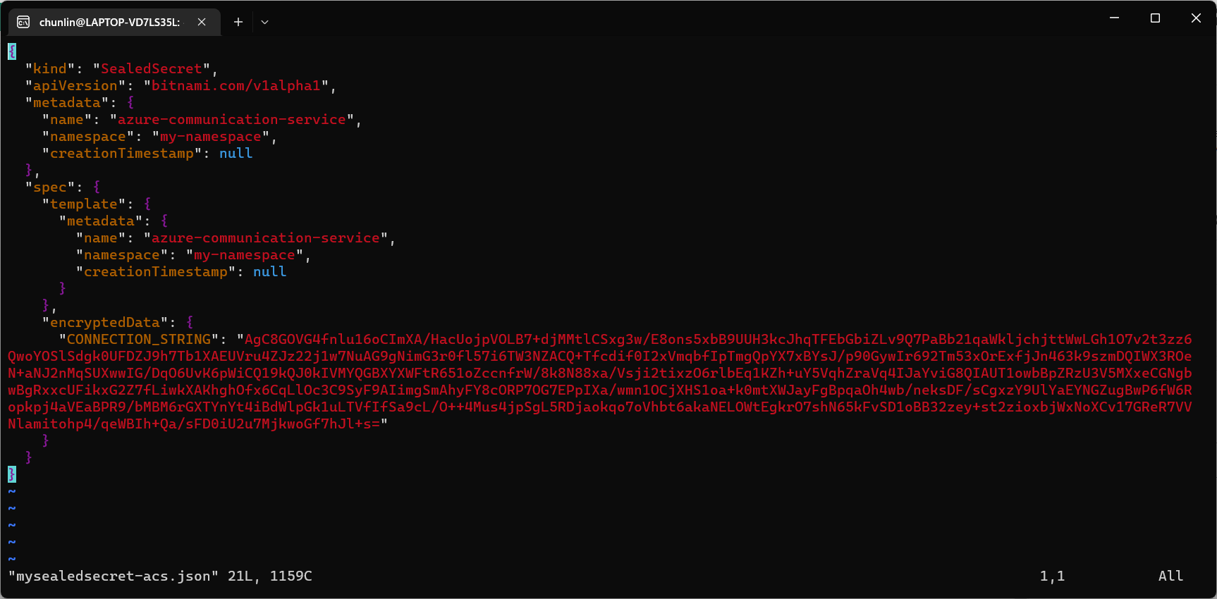
kubectl create secret generic azure-communication-service --from-literal=CONNECTION_STRING=xxxxxx --dry-run=client --namespace=my-namespace -o json > mysecret-acs.json

kubeseal < mysecret-acs.json > mysealedsecret-acs.json
The generated file mysealedsecret-acs.json should look something as shown below.
To create the Secret resource, we will simply create it based on the file mysealedsecret-acs.json.
This generated file mysealedsecret-acs.json is thus safe to be committed to our code repository.
Going Zero-Trust: Using Kamus and InitContainer
Besides SealedSecret, there is also another open-source solution known as Kamus, a zero-trust secrets encryption and decryption solution for Kubernetes apps. We can also use Kamus to encrypt our secrets and make sure that the secrets can only be decrypted by the desired Kubernetes apps.
Similarly, we can also install Kamus using Helm Chart with the commands below.
helm repo add soluto https://charts.soluto.io
helm upgrade --install kamus soluto/kamus
Kamus will encrypt secrets for only a specific application represented by a ServiceAccount. A service account provides an identity for processes that run in a Pod, and maps to a ServiceAccount object. Hence, we need to create a Service Account with the YAML below.
apiVersion: v1
kind: ServiceAccount
metadata:
  name: my-kamus-sa
After creating the ServiceAccount, we can update our CronJob YAML to mount it on the pods.
Next, we can proceed to download and install Kamus CLI which we can use to encrypt our secret with the following command.
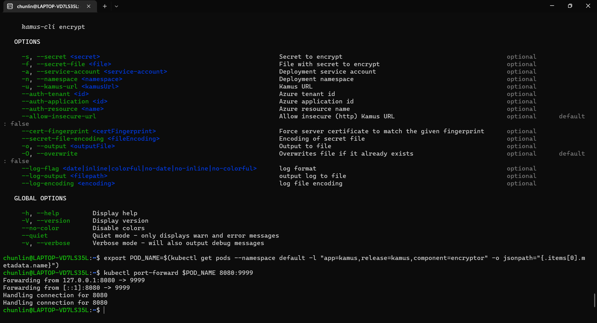
kamus-cli encrypt \
  --secret xxxxxxxx \
  --service-account my-kamus-sa \
  --namespace my-namespace \
  --kamus-url <Kamus URL>
The Kamus URL could be found after we installed Kamus as shown in the screenshot below.

We need to follow the instruction printed on the screen to get the Kamus URL. To do so, we need to forward local port to the pod, as shown in the following screenshot.
Hence, let’s say we want to encrypt a secret “alamak”, we can do so as follows.
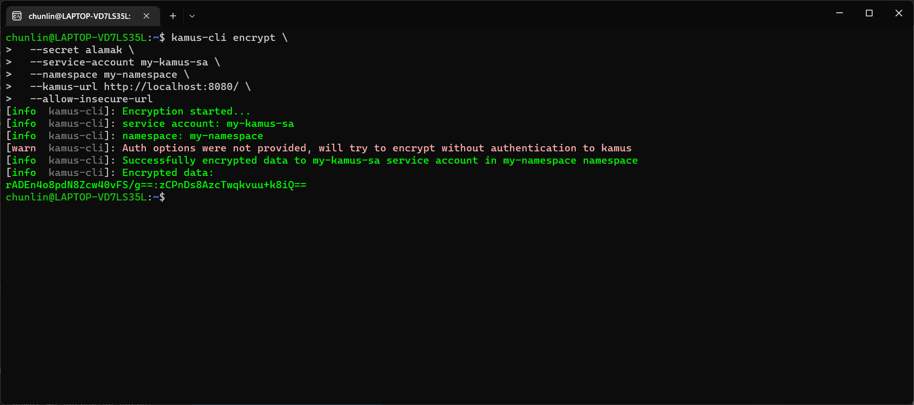
After we have encrypted our secret successfully, we need to configure our pod accordingly so that it can decrypt the value with Kamus Decrypt API. The simplest way will be storing our secret in a ConfigMap because it is already encrypted, so it’s safe to store it in ConfigMap.
apiVersion: v1
kind: ConfigMap
metadata:
  name: my-encrypted-secret
  namespace: my-namespace
data:
  data: rADEn4o8pdN8Zcw40vFS/g==:zCPnDs8AzcTwqkvuu+k8iQ==
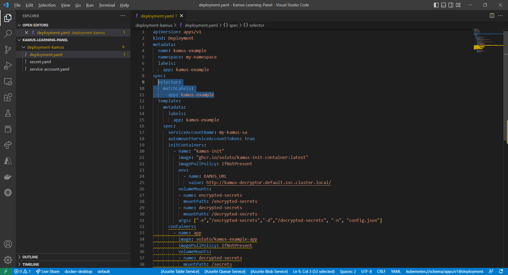
Then we can include an InitContainer in our pod. This is because the use of an initContainer allows one or more containers to run only if one or more previous containers run and exit successfully. So we can make use of Kamus Init Container to decrypt the secret using Kamus Decryptor API and output it to a file to be consumed by our app. There is an official demo from the Kamus Team on how to do that on the GitHub. Please take note that one of their YAML files is outdated and thus there is a need to update their deployment.yaml to use “apiVersion: apps/v1” with a proper selector.
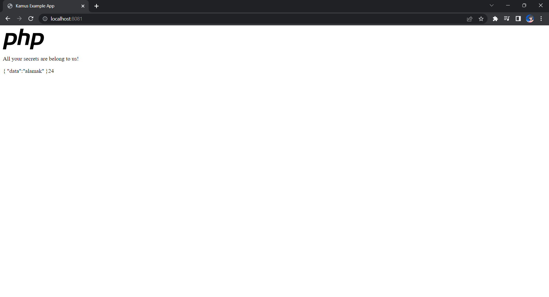
After the deployment is successful, we can forward the port 8081 to the pod in the deployment as shown below.
kubectl port-forward deployment/kamus-example 8081:80
If the deployment is successful, we should be able to see the following when we visit localhost:8081 on our Internet browser, as shown in the following screenshot.
Deploy Our CronJob
Now, since we have everything setup, we can create our Kubernetes CronJob with the YAML file we have earlier. For local testing, I have edited the schedule to be “*/2 * * * *”. This means that an email will be sent to me every 2 minutes.
After waiting for a couple of minutes, I have received a few emails sent via the Azure Communication Services, as shown below.
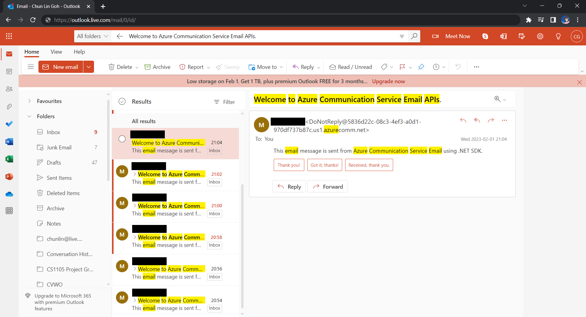
Hoorey, this is how we build a simple Kubernetes CronJob and how we can send emails with the Azure Email Communication Services.