In our previous post, we introduced SilverVector as a “Day 0” dashboard prototyping tool. Today, we are going to show you exactly how powerful that can be by applying it to a real-world, complex open-source CMS: Orchard Core.
Orchard Core is a fantastic, modular CMS built on ASP.NET Core. It is powerful, flexible, and used by enterprises worldwide. However, because it is so flexible, monitoring it on dashboard like Grafana can be a challenge. Orchard Core stores content as JSON documents, which means “simple” questions like “How many articles did we publish today?” often require complex queries or custom admin modules.
With SilverVector, we solved this in seconds.
Grafana: Your open and composable observability stack. (Event Page)
The “Few Clicks” Promise
Usually, building a dashboard for a CMS like Orchard Core involves:
Installing a monitoring plugin (if one exists).
Configuring Prometheus exporters.
Building panels manually in Grafana.
With SilverVector, we took a different approach. We simply asked: “What does the database look like?”
We took the standard SQL file containing Orchard Core DDL, i.e the script that creates the database tables used in the CMS. We did not need to connect to a live server. We also did not need API keys. We just needed the schema.
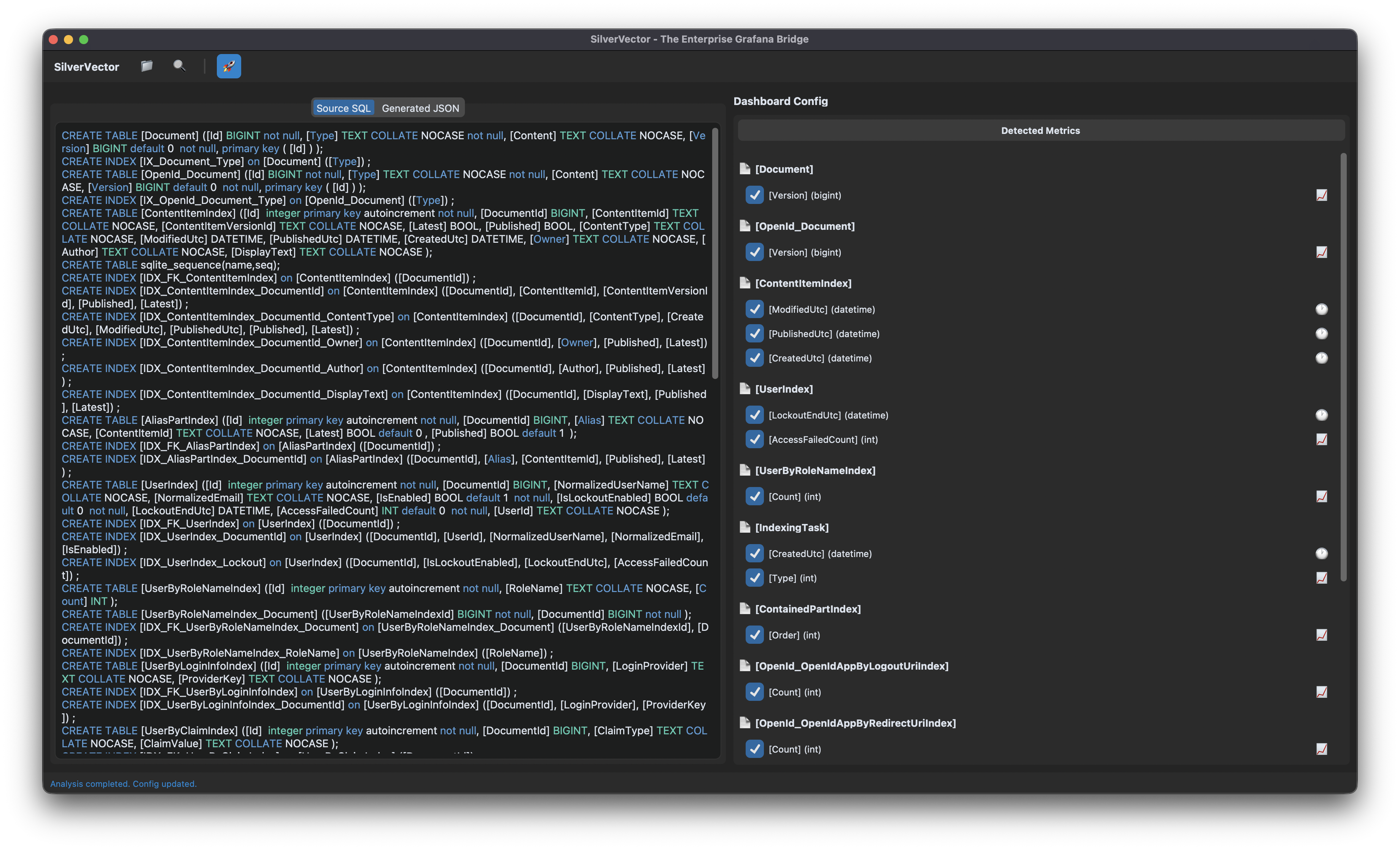
We taught SilverVector to recognise the signature of an Orchard Core database.
It sees ContentItemIndex? It knows this is an Orchard Core CMS;
It sees UserIndex? It knows there are users to count;
It sees PublishedUtc? It knows we can track velocity.
SilverVector detects the relevant metrics from the Orchard Core DDL that could be used in Grafana dashboard.
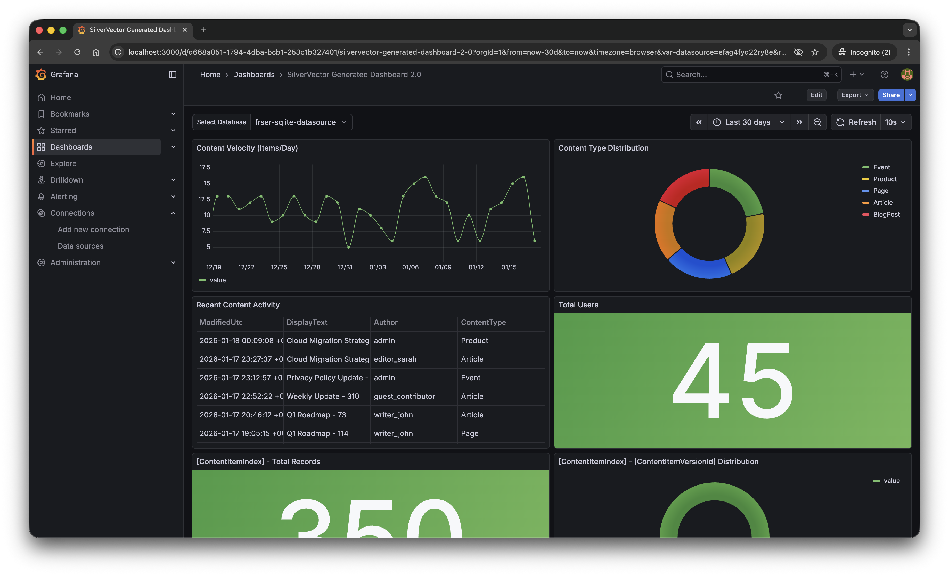
With a single click of the “blue rocket” button, SilverVector generated a JSON dashboard pre-configured with:
Content Velocity: A time-series graph showing publishing trends over the last 30 days.
Content Distribution: A pie chart breaking down content by type (Articles, Products, Pages).
Recent Activity: A detailed table of who changed what and when.
User Growth: A stat panel showing the total registered user base.
The “Content Velocity” graph generated by SilverVector.
Why This Matters for Orchard Core Developers
This is not just about saving 10 minutes of clicking to setup the initial Grafana dashboard. It is about empowerment.
As Orchard Core developers, you do not need to commit to a complex observability stack just to see if it is worth it. You can generate this dashboard locally, just as demonstrated above, point it at a backup of your production database, and instantly show your stakeholders the value of your work.
For many small SMEs in Singapore and Malaysia, as shared in our earlier post, the barrier of deploying observability stack is not just technical but it is survival. They are often too busy worrying about the rent of this month to invest time in a complex tech stack they do not fully understand. SilverVector lowers that barrier to minimal.
SilverVector gives you the foundation. We generate the boring boilerplate, i.e. the grid layout, the panel IDs, the basic SQL queries. Once you have that JSON, you are free to extend it! For example, you want to add CPU Usage? Just add a panel for your server metrics. Want to track Page Views? Join it with your IIS/Nginx logs.
In addition, since we rely on standard SQL indices such as ContentItemIndex, this dashboard works on any Orchard Core installation that uses a SQL database (SQL Server, SQLite, PostgreSQL, MySQL). You do not need to install a special module in your CMS application code.
A Call to Action
We believe the “Day 0” of observability should not be hard. It should be a default.
If you are an Orchard Core developer, try SilverVector today. Paste in your DDL, generate the dashboard, and see your Orchard Core CMS in a whole new light.
SilverVector is open source. Fork it, tweak the detection logic, and help us build the ultimate “Day 0” dashboard tool for every developer.
In the world of data visualisation, Grafana is the leader. It is the gold standard for observability, used by industry leaders to monitor everything from bank transactions to Mars rovers. However, for a local e-commerce shop in Penang or a small digital agency in Singapore, Grafana can feel like bringing a rocket scientist tool to cut fruits because it is powerful, but perhaps too difficult to use.
This is why we build SilverVector.
SilverVector generates standard Grafana JSON from DDL.
Why SilverVector?
In Malaysia and Singapore, SMEs are going digital very fast. However, they rarely have a full DevOps team. Usually, they just rely on The Solo Engineer, i.e. the freelancer, the agency developer, or the “full-stack developer” who does everything.
A common mistake in growing SMEs is asking full-stack developers to build meaningful business insights. The result is almost always a custom-coded “Admin Panel”.
While functional, these custom tools are hidden technical debt:
High Maintenance: Every new metric requires a code change and a deployment;
Poor Performance: Custom dashboards are often unoptimised;
Lack of Standards: Every internal tool looks different.
Custom panels developed in-house in SMEs are often ugly, hard to maintain, and slow because they often lack proper pagination or caching.
SilverVector allows you to skip building the internal tool entirely. By treating Grafana as your GUI layer, you get a standardised, performant, and beautiful interface for free. You supply the SQL and Grafana handles the rendering.
In addition, to some of the full-stack developers, building a proper Grafana dashboard from scratch involves hours of repetitive GUI clicking.
For an SME, “Zero Orders in the last hour” is not just a statistic. Instead, it is an emergency. SilverVector focuses on this Operational Intelligence, helping backend engineers visualise their system health easily.
Why not just use Terraform?
Terraform (and GitOps) is the gold standard for long-term maintenance. But terraform import requires an existing resource. SilverVector acts as the prototyping engine. It helps us in Day 0, i.e. getting us from “Zero” to “First Draft” in a few seconds. Once the client approves the dashboard, we can export that JSON into our GitOps workflow. We handle the chaotic “Drafting Phase” so our Terraform manages the “Stable Phase.”
Another big problem is trust. In the enterprise world, shadow IT is a nightmare. In the SME world, managers are also afraid to give API keys or database passwords to a tool they just found on GitHub.
SilverVector was built on a strict “Zero-Knowledge” principle.
We do not ask for database passwords;
We do not ask for API keys;
We do not connect to your servers.
We only ask for one safe thing: Schema (DDL). By checking the structure of your data (like CREATE TABLE orders...) and not the meaningful data itself, we can generate the dashboard configuration file. You take that file and upload it to your own Grafana yourself. We never connect to your production environment.
Key Technical Implementation
Building this tool means we act like a translator: SQL DDL -> Grafana JSON Model. Here is how we did it.
We did not use a heavy full SQL engine because we are not trying to be a database. We simply want to be a shortcut.
We built SilverVectorParser using regex and simple logic to solve the “80/20” problem. It guesses likely metrics (e.g., column names like amount, duration) and dimensions. However, regex is not perfect. That is why the Tooling matters more than the Parser. If our logic guesses wrong, you do not have to debug our python code. You just uncheck the box in the UI.
The goal is not to be a perfect compiler. Instead, it is to be a smart assistant that types the repetitive parts for you.
Screenshot of the SilverVector UI Main Window.
For the interface, we choose CustomTkinter. Why a desktop GUI instead of a web app?
It comes down to Speed and Reality.
Offline-First: Network infrastructure in parts of Malaysia, from remote industrial sites in Sarawak to secure server basements in Johor Bahru can be spotty. This is critical for engineers deploying to Self-Hosted Grafana (OSS) instances where Internet access is restricted or unavailable;
Zero Configuration: Connecting a tool to your Grafana API requires generating service accounts, copying tokens, and configuring endpoints. It is tedious. SilverVector bypasses this “configuration tax” by generating a standard JSON file when you can just generate, drag, and drop.
Human-in-the-Loop: A command-line tool runs once and fails if the regex is wrong. Our UI allows you to see the detection and correct it instantly via checkboxes before generating the JSON.
To make the tool feel like a real developer product, we integrate a proper code experience. We use pygments to read both the input SQL and the output JSON. We then map those tokens to Tkinter text tags colours. This makes it look familiar, so you can spot syntax errors in the input schema easily.
Close-up zoom of the text editor area in SilverVector.
Technical Note: To ensure the output actually works when you import it:
Datasources: We set the Data Source as a Template Variable. On import, Grafana will simply ask you: “Which database do you want to use?” You do not need to edit the JSON helper IDs manually.
Performance: Time-series queries automatically include time range clauses (using $__from and $__to). This prevents the dashboard from accidentally scanning your entire 10-year history every time you refresh;
SQL Dialects: The current version uses SQLite for the local demo so anyone can test it immediately without spinning up Docker containers.
Future-Proofing for Growth
SilverVector is currently in its MVP phase, and the vision is simple: Productivity.
If you are a consultant or an engineer who has to set up observability for many projects, you know the pain of configuring panel positions manually. SilverVector is the painkiller. Stop writing thousands of lines of JSON boilerplate. Paste your schema, click generate, and spend your time on the queries that actually matter.
The resulting Grafana dashboard generated by SilverVector.
A sensible question that often comes up is: “Is this just a short-term fix? What happens when I hire a real team?”
The answer lies in Standardisation.
SilverVector generates standard Grafana JSON, which is the industry default. Since you own the output file, you will never be locked in to our tool.
Ownership: You can continue to edit the dashboard manually in Grafana OSS or Grafana Cloud as your requirements change;
Scalability: When you eventually hire a full DevOps engineer or migrate to Grafana Cloud, the JSON generated by SilverVector is fully compatible. You can easily convert it into advanced Code (like Terraform) later. We simply do the heavy lifting of writing the first 500 lines for them;
Stability: By building on simple SQL principles, the dashboard remains stable even as your data grows.
In addition, since SilverVector generates SQL queries that read from your database directly, you must be a responsible engineer to ensure your columns (especially timestamps) are indexed properly. A dashboard is only as fast as the database underneath it!
In short, we help you build the foundation quickly so you can renovate freely later.
In cloud infrastructure, the ultimate challenge is building systems that are not just resilient, but also radically efficient. We cannot afford to provision hardware for peak loads 24/7 because it is simply a waste of money.
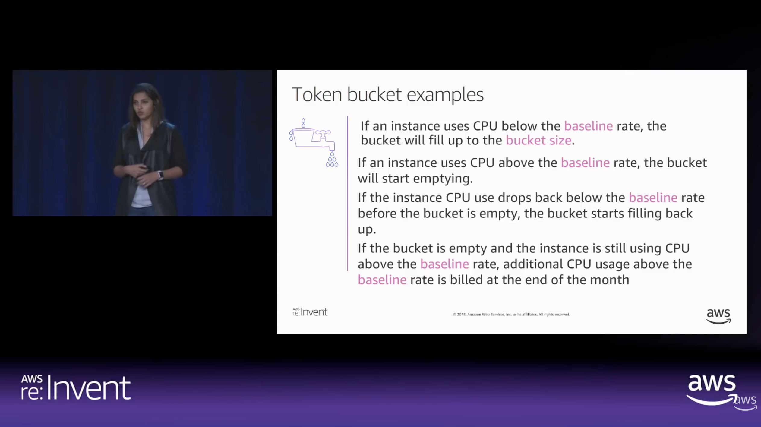
To achieve radical efficiency, AWS offers the T-series (like T3 and T4g). These instances allow us to pay for a baseline CPU level while retaining the ability to “burst” during high-traffic periods. This performance is governed by CPU Credits.
Modern T3 instances run on the AWS Nitro System, which offloads I/O tasks. This means nearly 100% of the credits we burn are spent on our actual SQL queries rather than background noise.
By default, Amazon RDS T3 instances are configured for “Unlimited Mode”. This prevents our database from slowing down when credits hit zero, but it comes with a cost: We will be billed for the Surplus Credits.
How CPU Credits are earned vs. spent over time. (Source: AWS re:Invent 2018)
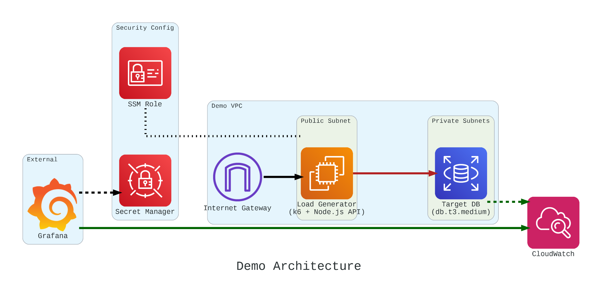
The Experiment: Designing the Stress Test
To truly understand how these credits behave under pressure, we built a controlled performance testing environment.
Our setup involved:
The Target: An Amazon RDS db.t3.medium instance.
The Generator: An EC2 instance running k6. We chose k6 because it allows us to write performance tests in JavaScript that are both developer-friendly and incredibly powerful.
The Workload: We simulated 200 concurrent users hitting an API that triggered heavy, CPU-bound SQL queries.
Simulation Fidelity with Micro-service
If we had k6 connect directly to PostgreSQL, it would not look like real production traffic. In order to make our stress test authentic, we introduce a simple NodeJS micro-service to act as the middleman.
This service does two critical things:
Implements a Connection Pool: Using the pg library Pool with a max: 20 setting, it mimics how a real-world app manages database resources;
Triggers the “Heavy Lifting”: The /heavy-query endpoint is designed to be purely CPU-bound. It forces the database to perform 1,000,000 calculations per request using nested generate_series.
In our k6 load test, we do not just flip a switch. We design a specific three-stage lifecycle for our RDS instance:
Ramp Up: We started with a gradual ramp-up from 0 to 50 users. This allows the connection pool to warm up and ensures we are not seeing performance spikes just from initial handshakes;
High-load Burn: We push the target to 200 concurrent users. These users will be hitting a /heavy-query endpoint that forces the database to calculate a million rows per second. This stage is designed to drain the CPUCreditBalance and prove that “efficiency” has its limits;
Ramp Down: Finally, we ramp back down to zero. This is the crucial moment in Grafana where we watch to see if the CPU credits begin to accumulate again or if the instance remains in a “debt” state.
import http from 'k6/http'; import { check, sleep } from 'k6';
export default function () { const res = http.get('http://localhost:3000/heavy-query'); check(res, { 'status was 200': (r) => r.status == 200 }); sleep(0.1); }
Monitoring with Grafana
If we are earning CPU credits slower than we are burning them, we are effectively walking toward a performance (or financial) cliff. To be truly resilient, we must monitor our CPUCreditBalance.
We use Grafana to transform raw CloudWatch signals into a peaceful dashboard. While “Unlimited Mode” keeps the latency flat, Grafana reveals the truth: Our credit balance decreases rapidly when CPU utilisation goes up to 100%.
Grafana showing the inverse relationship between high CPU Utilisation and a dropping CPU Credit Balance.
Predicting the Future with Discrete Event Simulation
Physical load testing with k6 is essential, but it takes real-time to run and costs real money for instance uptime.
Simulate a 24-hour traffic spike in just a few seconds;
Mathematically prove whether a rds.t3.medium is more cost-effective for a specific workload;
Predict exactly when an instance will run out of credits before we ever deploy it.
Simulation results from the SNA.
Final Thoughts
Efficiency is not just about saving money. Instead, it is about understanding the mathematical limits of our architecture. By combining AWS burstable instances with deep observability and predictive discrete event simulation, we can build systems that are both lean and unbreakable.
For those interested in the math behind the simulation, check out the SNA Library on GitHub.
In the previous article, we have discussed about how we can build a custom monitoring pipeline that has Grafana running on Amazon ECS to receive metrics and logs, which are two of the observability pillars, sent from the Orchard Core on Amazon ECS. Today, we will proceed to talk about the third pillar of observability, traces.
Source Code
The CloudFormation templates and relevant C# source codes discussed in this article is available on GitHub as part of the Orchard Core Basics Companion (OCBC) Project:https://github.com/gcl-team/Experiment.OrchardCore.Main.
Lisa Jung, senior developer advocate at Grafana, talks about the three pillars in observability (Image Credit: Grafana Labs)
We choose Tempo because it is fully compatible with OpenTelemetry, the open standard for collecting distributed traces, which ensures flexibility and vendor neutrality. In addition, Tempo seamlessly integrates with Grafana, allowing us to visualise traces alongside metrics and logs in a single dashboard.
Finally, being a Grafana Labs project means Tempo has strong community backing and continuous development.
About OpenTelemetry
With a solid understanding of why Tempo is our tracing backend of choice, let’s now dive deeper into OpenTelemetry, the open-source framework we use to instrument our Orchard Core app and generate the trace data Tempo collects.
OpenTelemetry is a Cloud Native Computing Foundation (CNCF) project and a vendor-neutral, open standard for collecting traces, metrics, and logs from our apps. This makes it an ideal choice for building a flexible observability pipeline.
OpenTelemetry provides SDKs for instrumenting apps across many programming languages, including C# via the .NET SDK, which we use for Orchard Core.
OpenTelemetry uses the standard OTLP (OpenTelemetry Protocol) to send telemetry data to any compatible backend, such as Tempo, allowing seamless integration and interoperability.
The http_listen_port allows us to set the HTTP port (3200) for Tempo internal web server. This port is used for health checks and Prometheus metrics.
After that, we configure where Tempo listens for incoming trace data. In the configuration above, we enabled OTLP receivers via both gRPC and HTTP, the two protocols that OpenTelemetry SDKs and agents use to send data to Tempo. Here, the ports 4317 (gRPC) and 4318 (HTTP) are standard for OTLP.
Last but not least, in the configuration, as demonstration purpose, we use the simplest one, local storage, to write trace data to the EC2 instance disk under /tmp/tempo/traces. This is fine for testing or small setups, but for production we will likely want to use services like Amazon S3.
In addition, since we are using local storage on EC2, we can easily SSH into the EC2 instance and directly inspect whether traces are being written. This is incredibly helpful during debugging. What we need to do is to run the following command to see whether files are being generated when our Orchard Core app emits traces.
ls -R /tmp/tempo/traces
The configuration above is intentionally minimal. As our setup grows, we can explore advanced options like remote storage, multi-tenancy, or even scaling with Tempo components.
Each flushed trace block (folder with UUID) contains a data.parquet file, which holds the actual trace data.
Finally, in order to enable Tempo to start on boot, we create a systemd unit file that allows Tempo to start on boot and automatically restart if it crashes.
cat <<EOF > /etc/systemd/system/tempo.service [Unit] Description=Grafana Tempo service After=network.target
systemctl daemon-reexec systemctl daemon-reload systemctl enable --now tempo
This systemd service ensures that Tempo runs in the background and automatically starts up after a reboot or a crash. This setup is crucial for a resilient observability pipeline.
Did You Know: When we SSH into an EC2 instance running Amazon Linux 2023, we will be greeted by a cockatiel in ASCII art! (Image Credit: OMG! Linux)
Understanding OTLP Transport Protocols
In the previous section, we configured Tempo to receive OTLP data over both gRPC and HTTP. These two transport protocols are supported by the OTLP, and each comes with its own strengths and trade-offs. Let’s break them down.
Ivy Zhuang from Google gave a presentation on gRPC and Protobuf at gRPConf 2024. (Image Credit: gRPC YouTube)
Tempo has native support for gRPC, and many OpenTelemetry SDKs default to using it. gRPC is a modern, high-performance transport protocol built on top of HTTP/2. It is the preferred option when performanceis critical. gRPC also supports streaming, which makes it ideal for high-throughput scenarios where telemetry data is sent continuously.
However, gRPC is not natively supported in browsers, so it is not ideal for frontend or web-based telemetry collection unless a proxy or gateway is used. In such scenarios, we will normally choose HTTP which is browser-friendly. HTTP is a more traditional request/response protocol that works well in restricted environments.
Since we are collecting telemetry from server-side like Orchard Core running on ECS, gRPC is typically the better choice due to its performance benefits and native support in Tempo.
Please take note that since gRPC requires HTTP/2, which some environments, for example, IoT devices and embedding systems, might not have mature gRPC client support, OTLP over HTTP is often preferred in simpler or constrained systems.
gRPC allows multiplexing over a single connection using HTTP/2. Hence, in gRPC, all telemetry signals, i.e. logs, metrics, and traces, can be sent concurrently over one connection. However, with HTTP, each telemetry signal needs a separate POST request to its own endpoint as listed below to enforce clean schema boundaries, simplify implementation, and stay aligned with HTTP semantics.
Logs:/v1/logs;
Metrics:/v1/metrics;
Traces:/v1/traces.
In HTTP, since each signal has its own POST endpoint with its own protobuf schema in the body, there is no need for the receiver to guess what is in the body.
AWS Distro for Open Telemetry (ADOT)
Now that we have Tempo running on EC2 and understand the OTLP protocols it supports, the next step is to instrument our Orchard Core to generate and send trace data.
The following code snippet shows what a typical direct integration with Tempo might look like in an Orchard Core.
This approach works well for simple use cases during development stage, but it comes with trade-offs that are worth considering. Firstly, we couple our app directly to the observability backend, reducing flexibility. Secondly, central management becomes harder when we scale to many services or environments.
ADOT is a secure, AWS-supported distribution of the OpenTelemetry project that simplifies collecting and exporting telemetry data from apps running on AWS services, for example our Orchard Core on ECS now. ADOT decouples our apps from the observability backend, provides centralised configuration, and handles telemetry collection more efficiently.
Sidecar Pattern
We can deploy the ADOT in several ways, such as running it on a dedicated node or ECS service to receive telemetry from multiple apps. We can also take the sidecar approach which cleanly separates concerns. Our Orchard Core app will focus on business logic, while a nearby ADOT sidecar handles telemetry collection and forwarding. This mirrors modern cloud-native patterns and gives us more flexibility down the road.
The following CloudFormation template shows how we deploy ADOT as a sidecar in ECS using CloudFormation. The collector config is stored in AWS Systems Manager Parameter Store under /myapp/otel-collector-config, and injected via the AOT_CONFIG_CONTENT environment variable. This keeps our infrastructure clean, decoupled, and secure.
Deploy an ADOT sidecar on ECS to collect observability data from Orchard Core.
There are several interesting and important details in the CloudFormation snippet above that are worth calling out. Let’s break them down one by one.
Firstly, we choose awsvpc as the NetworkMode of the ECS task. In awsvpc, each container in the ECS task, i.e. our Orchard Core container and the ADOT sidecar, receives its own ENI (Elastic Network Interface). This is great for network-level isolation. With this setup, we can reference the sidecar from our Orchard Core using its container name through ECS internal DNS, i.e. http://adot-collector:4317.
Secondly, we include a health check for the ADOT container. ECS will use this health check to restart the container if it becomes unhealthy, improving reliability without manual intervention. In November 2022, Paurush Garg from AWS added the healthcheck component with the new ADOT collector release, so we can simply specify that we will be using this healthcheck component in the configuration that we will discuss next.
Yes, the configuration! Instead of hardcoding the ADOT configuration into the task definition, we inject it securely at runtime using the AOT_CONFIG_CONTENT secret. This environment variable AOT_CONFIG_CONTENT is designed to enable us to configure the ADOT collector. It will override the config file used in the ADOT collector entrypoint command.
The SSM Parameter for the environment variable AOT_CONFIG_CONTENT.
Wrap-Up
By now, we have completed the journey of setting up Grafana Tempo on EC2, exploring how traces flow through OTLP protocols like gRPC and HTTP, and understanding why ADOT is often the better choice in production-grade observability pipelines.
With everything connected, our Orchard Core app is now able to send traces into Tempo reliably. This will give us end-to-end visibility with OpenTelemetry and AWS-native tooling.