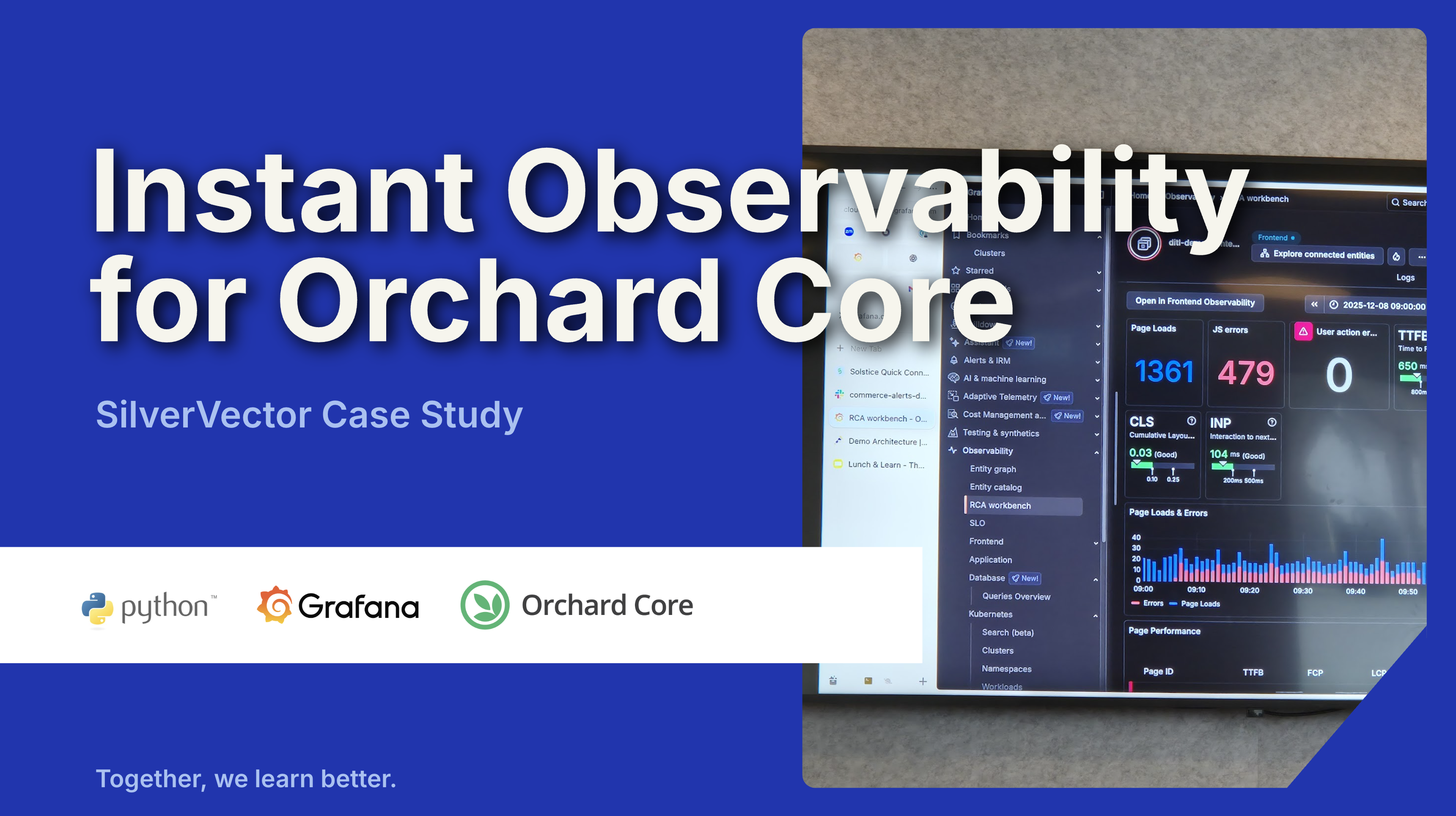
In our previous post, we introduced SilverVector as a “Day 0” dashboard prototyping tool. Today, we are going to show you exactly how powerful that can be by applying it to a real-world, complex open-source CMS: Orchard Core.
Orchard Core is a fantastic, modular CMS built on ASP.NET Core. It is powerful, flexible, and used by enterprises worldwide. However, because it is so flexible, monitoring it on dashboard like Grafana can be a challenge. Orchard Core stores content as JSON documents, which means “simple” questions like “How many articles did we publish today?” often require complex queries or custom admin modules.
With SilverVector, we solved this in seconds.
Grafana: Your open and composable observability stack. (Event Page)
The “Few Clicks” Promise
Usually, building a dashboard for a CMS like Orchard Core involves:
Installing a monitoring plugin (if one exists).
Configuring Prometheus exporters.
Building panels manually in Grafana.
With SilverVector, we took a different approach. We simply asked: “What does the database look like?”
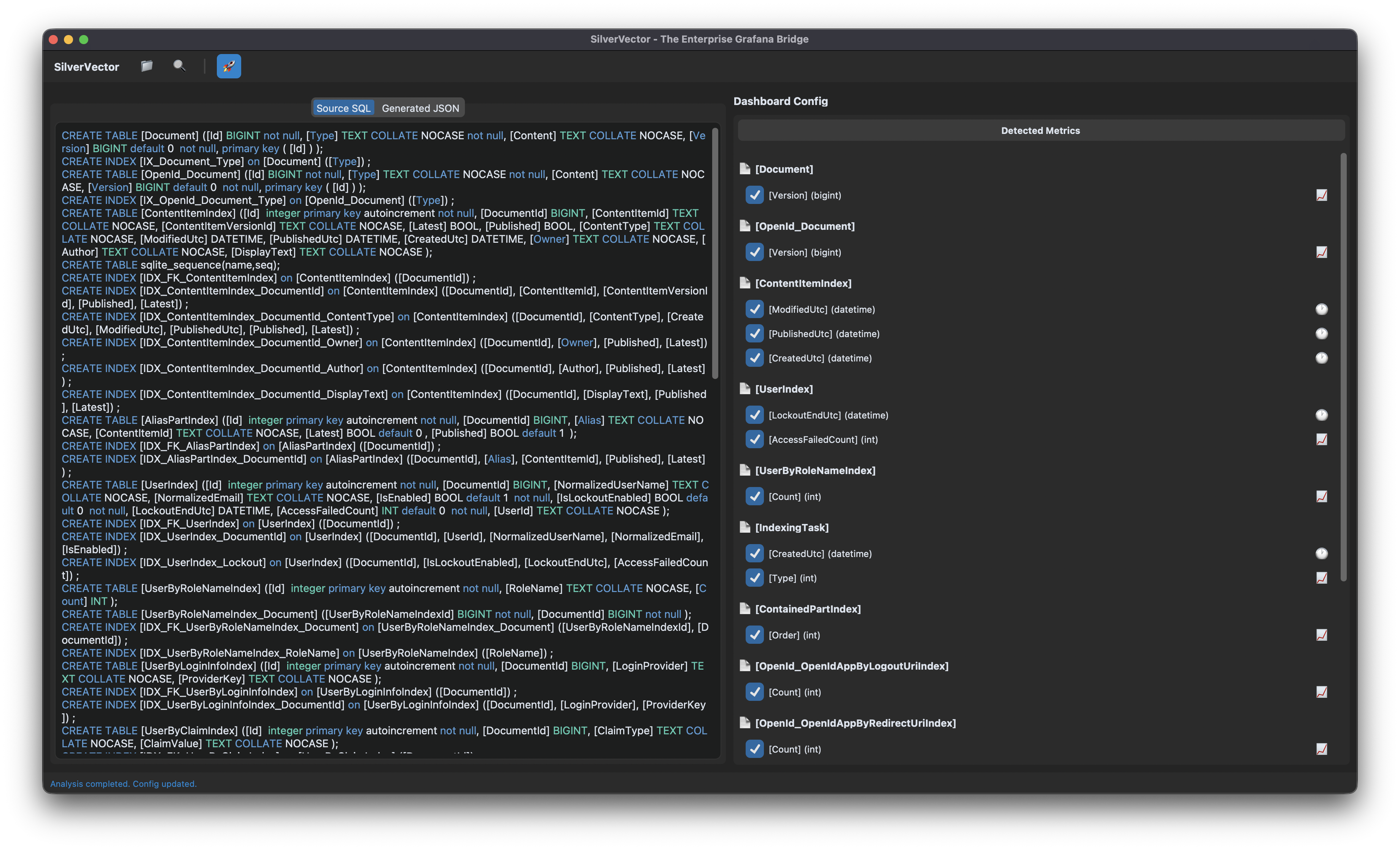
We took the standard SQL file containing Orchard Core DDL, i.e the script that creates the database tables used in the CMS. We did not need to connect to a live server. We also did not need API keys. We just needed the schema.
We taught SilverVector to recognise the signature of an Orchard Core database.
It sees ContentItemIndex? It knows this is an Orchard Core CMS;
It sees UserIndex? It knows there are users to count;
It sees PublishedUtc? It knows we can track velocity.
SilverVector detects the relevant metrics from the Orchard Core DDL that could be used in Grafana dashboard.
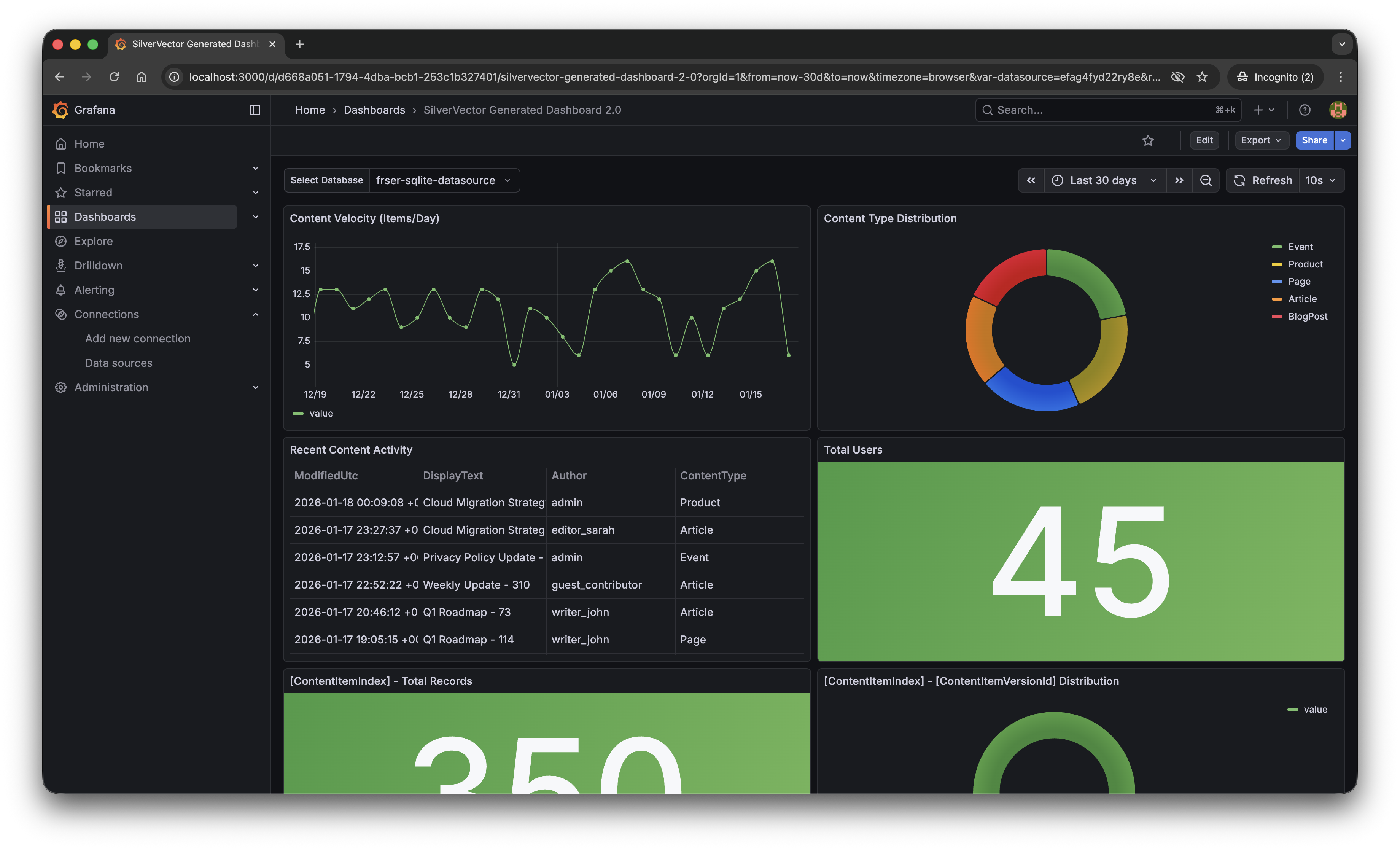
With a single click of the “blue rocket” button, SilverVector generated a JSON dashboard pre-configured with:
Content Velocity: A time-series graph showing publishing trends over the last 30 days.
Content Distribution: A pie chart breaking down content by type (Articles, Products, Pages).
Recent Activity: A detailed table of who changed what and when.
User Growth: A stat panel showing the total registered user base.
The “Content Velocity” graph generated by SilverVector.
Why This Matters for Orchard Core Developers
This is not just about saving 10 minutes of clicking to setup the initial Grafana dashboard. It is about empowerment.
As Orchard Core developers, you do not need to commit to a complex observability stack just to see if it is worth it. You can generate this dashboard locally, just as demonstrated above, point it at a backup of your production database, and instantly show your stakeholders the value of your work.
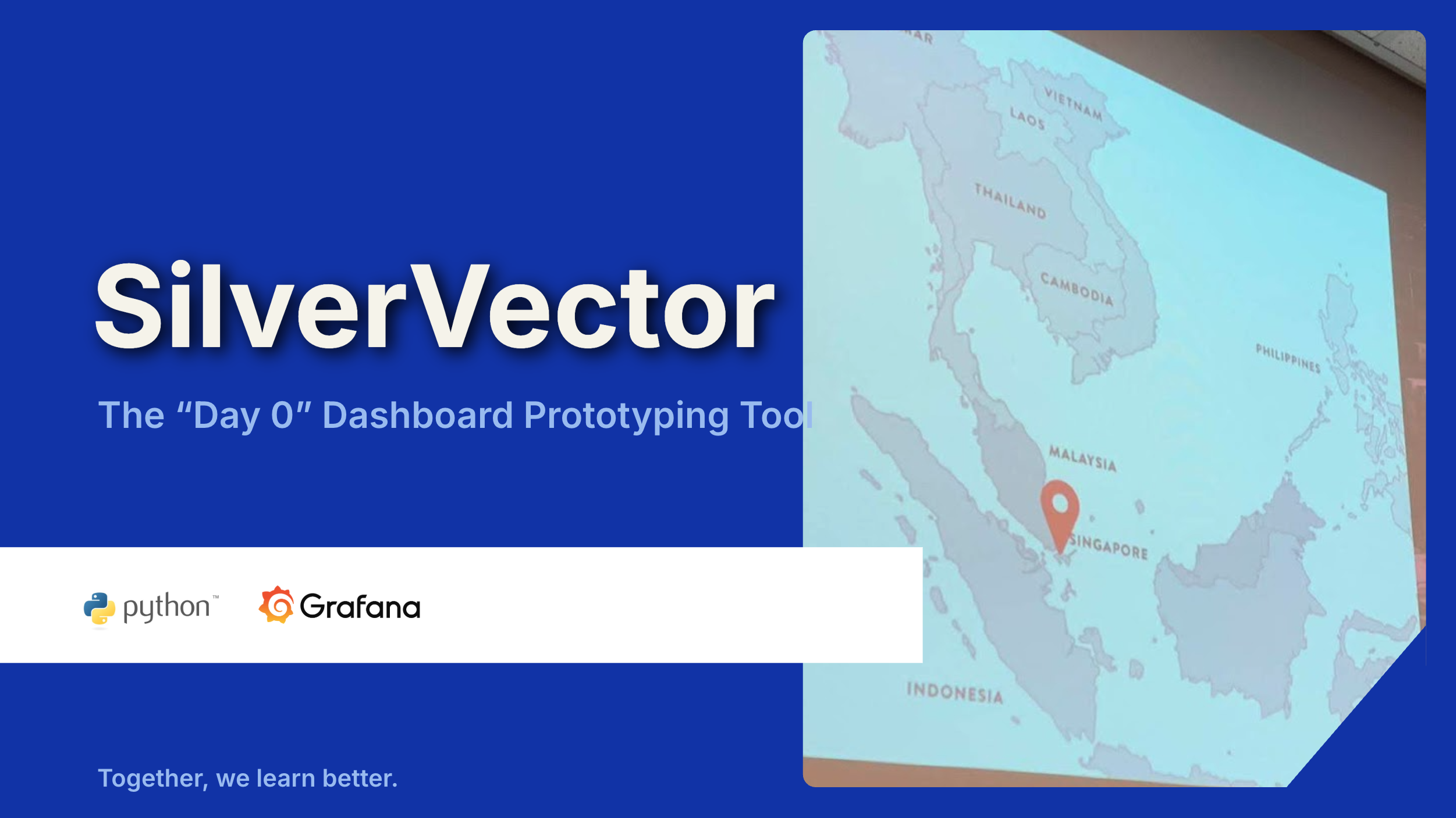
For many small SMEs in Singapore and Malaysia, as shared in our earlier post, the barrier of deploying observability stack is not just technical but it is survival. They are often too busy worrying about the rent of this month to invest time in a complex tech stack they do not fully understand. SilverVector lowers that barrier to minimal.
SilverVector gives you the foundation. We generate the boring boilerplate, i.e. the grid layout, the panel IDs, the basic SQL queries. Once you have that JSON, you are free to extend it! For example, you want to add CPU Usage? Just add a panel for your server metrics. Want to track Page Views? Join it with your IIS/Nginx logs.
In addition, since we rely on standard SQL indices such as ContentItemIndex, this dashboard works on any Orchard Core installation that uses a SQL database (SQL Server, SQLite, PostgreSQL, MySQL). You do not need to install a special module in your CMS application code.
A Call to Action
We believe the “Day 0” of observability should not be hard. It should be a default.
If you are an Orchard Core developer, try SilverVector today. Paste in your DDL, generate the dashboard, and see your Orchard Core CMS in a whole new light.
SilverVector is open source. Fork it, tweak the detection logic, and help us build the ultimate “Day 0” dashboard tool for every developer.
In the world of data visualisation, Grafana is the leader. It is the gold standard for observability, used by industry leaders to monitor everything from bank transactions to Mars rovers. However, for a local e-commerce shop in Penang or a small digital agency in Singapore, Grafana can feel like bringing a rocket scientist tool to cut fruits because it is powerful, but perhaps too difficult to use.
This is why we build SilverVector.
SilverVector generates standard Grafana JSON from DDL.
Why SilverVector?
In Malaysia and Singapore, SMEs are going digital very fast. However, they rarely have a full DevOps team. Usually, they just rely on The Solo Engineer, i.e. the freelancer, the agency developer, or the “full-stack developer” who does everything.
A common mistake in growing SMEs is asking full-stack developers to build meaningful business insights. The result is almost always a custom-coded “Admin Panel”.
While functional, these custom tools are hidden technical debt:
High Maintenance: Every new metric requires a code change and a deployment;
Poor Performance: Custom dashboards are often unoptimised;
Lack of Standards: Every internal tool looks different.
Custom panels developed in-house in SMEs are often ugly, hard to maintain, and slow because they often lack proper pagination or caching.
SilverVector allows you to skip building the internal tool entirely. By treating Grafana as your GUI layer, you get a standardised, performant, and beautiful interface for free. You supply the SQL and Grafana handles the rendering.
In addition, to some of the full-stack developers, building a proper Grafana dashboard from scratch involves hours of repetitive GUI clicking.
For an SME, “Zero Orders in the last hour” is not just a statistic. Instead, it is an emergency. SilverVector focuses on this Operational Intelligence, helping backend engineers visualise their system health easily.
Why not just use Terraform?
Terraform (and GitOps) is the gold standard for long-term maintenance. But terraform import requires an existing resource. SilverVector acts as the prototyping engine. It helps us in Day 0, i.e. getting us from “Zero” to “First Draft” in a few seconds. Once the client approves the dashboard, we can export that JSON into our GitOps workflow. We handle the chaotic “Drafting Phase” so our Terraform manages the “Stable Phase.”
Another big problem is trust. In the enterprise world, shadow IT is a nightmare. In the SME world, managers are also afraid to give API keys or database passwords to a tool they just found on GitHub.
SilverVector was built on a strict “Zero-Knowledge” principle.
We do not ask for database passwords;
We do not ask for API keys;
We do not connect to your servers.
We only ask for one safe thing: Schema (DDL). By checking the structure of your data (like CREATE TABLE orders...) and not the meaningful data itself, we can generate the dashboard configuration file. You take that file and upload it to your own Grafana yourself. We never connect to your production environment.
Key Technical Implementation
Building this tool means we act like a translator: SQL DDL -> Grafana JSON Model. Here is how we did it.
We did not use a heavy full SQL engine because we are not trying to be a database. We simply want to be a shortcut.
We built SilverVectorParser using regex and simple logic to solve the “80/20” problem. It guesses likely metrics (e.g., column names like amount, duration) and dimensions. However, regex is not perfect. That is why the Tooling matters more than the Parser. If our logic guesses wrong, you do not have to debug our python code. You just uncheck the box in the UI.
The goal is not to be a perfect compiler. Instead, it is to be a smart assistant that types the repetitive parts for you.
Screenshot of the SilverVector UI Main Window.
For the interface, we choose CustomTkinter. Why a desktop GUI instead of a web app?
It comes down to Speed and Reality.
Offline-First: Network infrastructure in parts of Malaysia, from remote industrial sites in Sarawak to secure server basements in Johor Bahru can be spotty. This is critical for engineers deploying to Self-Hosted Grafana (OSS) instances where Internet access is restricted or unavailable;
Zero Configuration: Connecting a tool to your Grafana API requires generating service accounts, copying tokens, and configuring endpoints. It is tedious. SilverVector bypasses this “configuration tax” by generating a standard JSON file when you can just generate, drag, and drop.
Human-in-the-Loop: A command-line tool runs once and fails if the regex is wrong. Our UI allows you to see the detection and correct it instantly via checkboxes before generating the JSON.
To make the tool feel like a real developer product, we integrate a proper code experience. We use pygments to read both the input SQL and the output JSON. We then map those tokens to Tkinter text tags colours. This makes it look familiar, so you can spot syntax errors in the input schema easily.
Close-up zoom of the text editor area in SilverVector.
Technical Note: To ensure the output actually works when you import it:
Datasources: We set the Data Source as a Template Variable. On import, Grafana will simply ask you: “Which database do you want to use?” You do not need to edit the JSON helper IDs manually.
Performance: Time-series queries automatically include time range clauses (using $__from and $__to). This prevents the dashboard from accidentally scanning your entire 10-year history every time you refresh;
SQL Dialects: The current version uses SQLite for the local demo so anyone can test it immediately without spinning up Docker containers.
Future-Proofing for Growth
SilverVector is currently in its MVP phase, and the vision is simple: Productivity.
If you are a consultant or an engineer who has to set up observability for many projects, you know the pain of configuring panel positions manually. SilverVector is the painkiller. Stop writing thousands of lines of JSON boilerplate. Paste your schema, click generate, and spend your time on the queries that actually matter.
The resulting Grafana dashboard generated by SilverVector.
A sensible question that often comes up is: “Is this just a short-term fix? What happens when I hire a real team?”
The answer lies in Standardisation.
SilverVector generates standard Grafana JSON, which is the industry default. Since you own the output file, you will never be locked in to our tool.
Ownership: You can continue to edit the dashboard manually in Grafana OSS or Grafana Cloud as your requirements change;
Scalability: When you eventually hire a full DevOps engineer or migrate to Grafana Cloud, the JSON generated by SilverVector is fully compatible. You can easily convert it into advanced Code (like Terraform) later. We simply do the heavy lifting of writing the first 500 lines for them;
Stability: By building on simple SQL principles, the dashboard remains stable even as your data grows.
In addition, since SilverVector generates SQL queries that read from your database directly, you must be a responsible engineer to ensure your columns (especially timestamps) are indexed properly. A dashboard is only as fast as the database underneath it!
In short, we help you build the foundation quickly so you can renovate freely later.
In cloud infrastructure, the ultimate challenge is building systems that are not just resilient, but also radically efficient. We cannot afford to provision hardware for peak loads 24/7 because it is simply a waste of money.
To achieve radical efficiency, AWS offers the T-series (like T3 and T4g). These instances allow us to pay for a baseline CPU level while retaining the ability to “burst” during high-traffic periods. This performance is governed by CPU Credits.
Modern T3 instances run on the AWS Nitro System, which offloads I/O tasks. This means nearly 100% of the credits we burn are spent on our actual SQL queries rather than background noise.
By default, Amazon RDS T3 instances are configured for “Unlimited Mode”. This prevents our database from slowing down when credits hit zero, but it comes with a cost: We will be billed for the Surplus Credits.
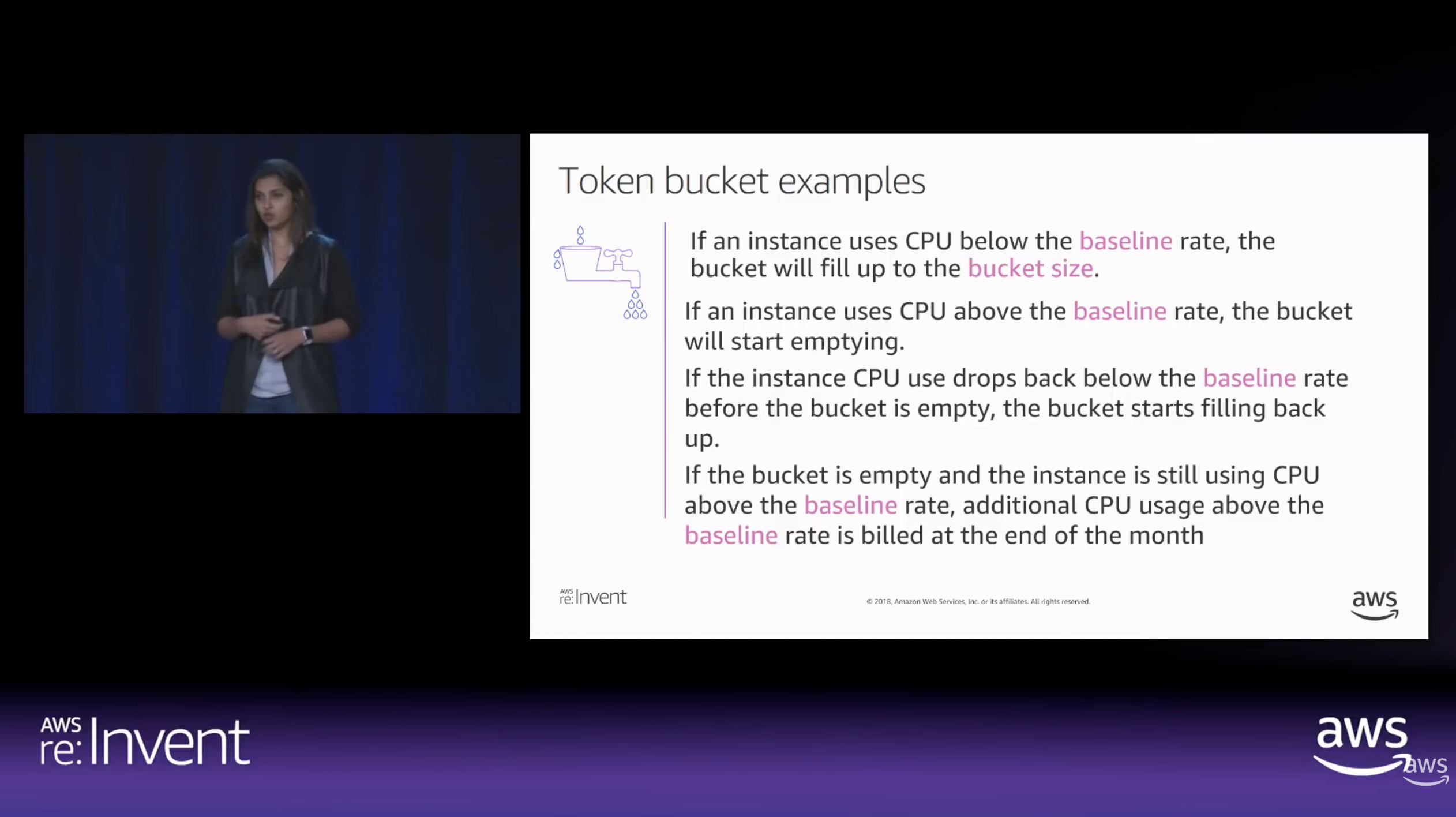
How CPU Credits are earned vs. spent over time. (Source: AWS re:Invent 2018)
The Experiment: Designing the Stress Test
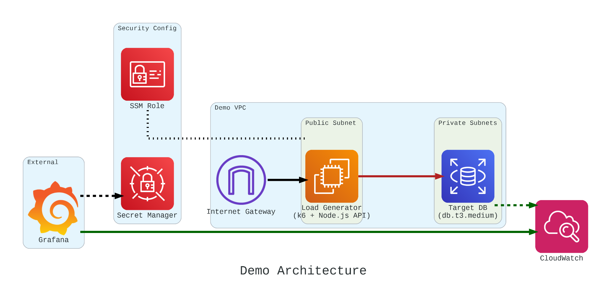
To truly understand how these credits behave under pressure, we built a controlled performance testing environment.
Our setup involved:
The Target: An Amazon RDS db.t3.medium instance.
The Generator: An EC2 instance running k6. We chose k6 because it allows us to write performance tests in JavaScript that are both developer-friendly and incredibly powerful.
The Workload: We simulated 200 concurrent users hitting an API that triggered heavy, CPU-bound SQL queries.
Simulation Fidelity with Micro-service
If we had k6 connect directly to PostgreSQL, it would not look like real production traffic. In order to make our stress test authentic, we introduce a simple NodeJS micro-service to act as the middleman.
This service does two critical things:
Implements a Connection Pool: Using the pg library Pool with a max: 20 setting, it mimics how a real-world app manages database resources;
Triggers the “Heavy Lifting”: The /heavy-query endpoint is designed to be purely CPU-bound. It forces the database to perform 1,000,000 calculations per request using nested generate_series.
In our k6 load test, we do not just flip a switch. We design a specific three-stage lifecycle for our RDS instance:
Ramp Up: We started with a gradual ramp-up from 0 to 50 users. This allows the connection pool to warm up and ensures we are not seeing performance spikes just from initial handshakes;
High-load Burn: We push the target to 200 concurrent users. These users will be hitting a /heavy-query endpoint that forces the database to calculate a million rows per second. This stage is designed to drain the CPUCreditBalance and prove that “efficiency” has its limits;
Ramp Down: Finally, we ramp back down to zero. This is the crucial moment in Grafana where we watch to see if the CPU credits begin to accumulate again or if the instance remains in a “debt” state.
import http from 'k6/http'; import { check, sleep } from 'k6';
export default function () { const res = http.get('http://localhost:3000/heavy-query'); check(res, { 'status was 200': (r) => r.status == 200 }); sleep(0.1); }
Monitoring with Grafana
If we are earning CPU credits slower than we are burning them, we are effectively walking toward a performance (or financial) cliff. To be truly resilient, we must monitor our CPUCreditBalance.
We use Grafana to transform raw CloudWatch signals into a peaceful dashboard. While “Unlimited Mode” keeps the latency flat, Grafana reveals the truth: Our credit balance decreases rapidly when CPU utilisation goes up to 100%.
Grafana showing the inverse relationship between high CPU Utilisation and a dropping CPU Credit Balance.
Predicting the Future with Discrete Event Simulation
Physical load testing with k6 is essential, but it takes real-time to run and costs real money for instance uptime.
Simulate a 24-hour traffic spike in just a few seconds;
Mathematically prove whether a rds.t3.medium is more cost-effective for a specific workload;
Predict exactly when an instance will run out of credits before we ever deploy it.
Simulation results from the SNA.
Final Thoughts
Efficiency is not just about saving money. Instead, it is about understanding the mathematical limits of our architecture. By combining AWS burstable instances with deep observability and predictive discrete event simulation, we can build systems that are both lean and unbreakable.
For those interested in the math behind the simulation, check out the SNA Library on GitHub.
I just spent two days at the Hello World Dev Conference 2025 in Taipei, and beneath the hype around cloud and AI, I observed a single, unifying theme: The industry is desperately building tools to cope with a complexity crisis of its own making.
The agenda was a catalog of modern systems engineering challenges. The most valuable sessions were the “踩雷經驗” (landmine-stepping experiences), which offered hard-won lessons from the front lines.
A 2-day technical conference on AI, Kubernetes, and more!
However, these talks raised a more fundamental question for me. We are getting exceptionally good at building tools to detect and recover from failure but are we getting any better at preventing it?
This post is not a simple translation of a Mandarin-language Taiwan conference. It is my analysis of the patterns I observed. I have grouped the key talks I attended into three areas:
Cloud Native Infrastructure;
Reshaping Product Management and Engineering Productivity with AI;
Deep Dives into Advanced AI Engineering.
Feel free to choose to dive into the section that interests you most.
Session: Smart Pizza and Data Observability
This session was led by Shuhsi (林樹熙), a Data Engineering Manager at Micron. Micron needs no introduction, they are a massive player in the semiconductor industry, and their smart manufacturing facilities are a prime example of where data engineering is mission-critical.
Shuhsi’s talk, “Data Observability by OpenLineage,” started with a simple story he called the “Smart Pizza” anomaly.
He presented a scenario familiar to anyone in a data-intensive environment: A critical dashboard flatlines, and the next three hours are a chaotic hunt to find out why. In his “Smart Pizza” example, the culprit was a silent, upstream schema change.
Smart pizza dashboard anomaly.
His solution, OpenLineage, is a powerful framework for what we would call digital forensics. It is about building a perfect, queryable map of the crime scene after the crime has been committed. By creating a clear data lineage, it reduces the “Mean Time to Discovery” from hours of panic to minutes of analysis.
Let’s be clear: This is critical, valuable work. Like OpenTelemetry for applications, OpenLineage brings desperately needed order to the chaos of modern data pipelines.
It is a fundamentally reactive posture. It helps us find the bullet path through the body with incredible speed and precision. However, my main point is that our ultimate goal must be to predict the bullet trajectory before the trigger is pulled. Data lineage minimises downtime. My work with simulation, which will be explained in the next session, aims to prevent it entirely by modelling these complex systems to find the breaking points before they break.
Session: Automating a .NET Discrete Event Simulation on Kubernetes
My talk, “Simulation Lab on Kubernetes: Automating .NET Parameter Sweeps,” addressed the wall that every complex systems analysis eventually hits: Combinatorial explosion.
While the industry is focused on understanding past failures, my session is about building the Discrete Event Simulation (DES) engine that can calculate and prevent future ones.
A restaurant simulation game in Honkai Impact 3rd. (Source: 西琳 – YouTube)
To make this concrete, I used the analogy of a restaurant owner asking, “Should I add another table or hire another waiter?” The only way to answer this rigorously is to simulate thousands of possible futures. The math becomes brutal, fast: testing 50 different configurations with 100 statistical runs each requires 5,000 independent simulations. This is not a task for a single machine; it requires a computational army.
My solution is to treat Kubernetes not as a service host, but as a temporary, on-demand supercomputer. The strategy I presented had three core pillars:
Declarative Orchestration: The entire 5,000-run DES experiment is defined in a single, clean Argo Workflows manifest, transforming a potential scripting nightmare into a manageable, observable process.
Radical Isolation: Each DES run is containerised in its own pod, creating a perfectly clean and reproducible experimental environment.
Controlled Randomness: A robust seeding strategy is implemented to ensure that “random” events in our DES are statistically valid and comparable across the entire distributed system.
The turnout for my DES session confirmed a growing hunger in our industry for proactive, simulation-driven approaches to engineering.
The final takeaway was a strategic re-framing of a tool many of us already use. Kubernetes is more than a platform for web apps. It can also be a general-purpose compute engine capable of solving massive scientific and financial modelling problems. It is time we started using it as such.
Session: AI for BI
Denny’s (監舜儀) session on “AI for BI” illustrated a classic pain point: The bottleneck between business users who need data and the IT teams who provide it. The proposed solution was a natural language interface, the FineChatBI, a tool designed to sit on top of existing BI platforms to make querying existing data easier.
Denny is introducing AI for BI.
His core insight was that the tool is the easy part. The real work is in building the “underground root system” which includes the immense challenge of defining metrics, managing permissions, and untangling data semantics. Without this foundation, any AI is doomed to fail.
Getting the underground root system right is important for building AI projects.
This is a crucial step forward in making our organisations more data-driven. However, we must also be clear about what problem is being solved.
This is a system designed to provide perfect, instantaneous answers to the question, “What happened?”
My work, and the next category of even more complex AI, begins where this leaves off. It seeks to answer the far harder question: “What will happen if…?” Sharpening our view of the past is essential, but the ultimate strategic advantage lies in the ability to accurately simulate the future.
Session: The Impossibility of Modeling Human Productivity
The presented Jugg (劉兆恭) is a well-known agile coach and the organiser of Agile Tour Taiwan 2020. His talk, “An AI-Driven Journey of Agile Product Development – From Inspiration to Delivery,” was a masterclass in moving beyond vanity metrics to understand and truly improve engineering performance.
Jugg started with a graph that every engineering lead knows in their gut. As a company grows over time:
Business grow (purple line, up);
Software architecture and complexity grow (first blue line, up);
The number of developers increases (second blue line, up);
Expected R&D productivity should grow (green line, up);
But paradoxically, the actual R&D productivity often stagnates or even declines (red line, down).
Jugg provided a perfect analogue for the work I do. He tackled the classic productivity paradox: Why does output stagnate even as teams grow? He correctly diagnosed the problem as a failure of measurement and proposed the SPACE framework as a more holistic model for this incredibly complex human system.
He was, in essence, trying to answer the same class of question I do: “If we change an input variable (team process), how can we predict the output (productivity)?”
This is where the analogy becomes a powerful contrast. Jugg’s world of human systems is filled with messy, unpredictable variables. His solutions are frameworks and dashboards. They are the best tools we have for a system that resists precise calculation.
This session reinforced my conviction that simulation is the most powerful tool we have for predicting performance in the systems we can actually control: Our code and our infrastructure. We do not have to settle for dashboards that show us the past because we can build models that calculate the future.
Session: Building a Map of “What Is” with GraphRAG
The most technically demanding session came from Nils (劉岦崱), a Senior Data Scientist at Cathay Financial Holdings. He presented GraphRAG, a significant evolution beyond the “Naive RAG” most of us use today.
Nils is explaining what a Naive RAG is.
He argued compellingly that simple vector search fails because it ignores relationships. By chunking documents, we destroy the contextual links between concepts. GraphRAG solves this by transforming unstructured data into a structured knowledge graph: a web of nodes (entities) and edges (their relationships).
Enhancing RAG-based application accuracy by constructing and leveraging knowledge graphs (Image Credit: LangChain)
In essence, GraphRAG is a sophisticated tool for building a static map of a known world. It answers the question, “How are all the pieces in our universe connected right now?” For AI customer service, this is a game-changer, as it provides a rich, interconnected context for every query.
This means our data now has an explicit, queryable structure. So, the LLM gets a much richer, more coherent picture of the situation, allowing it to maintain context over long conversations and answer complex, multi-faceted questions.
This session was a brilliant reminder that all advanced AI is built on a foundation of rigorous data modelling.
However, a map, no matter how detailed, is still just a snapshot. It shows us the layout of the city, but it cannot tell us how the traffic will flow at 5 PM.
This is the critical distinction. GraphRAG creates a model of a system at rest and DES creates a model of a system in motion. One shows us the relationships while the other lets us press watch how those relationships evolve and interact over time under stress. GraphRAG is the anatomy chart and simulation is the stress test.
Session: Securing the AI Magic Pocket with LLM Guardrails
Nils from Cathay Financial Holdings returned to the stage for Day 2, and this time he tackled one of the most pressing issues in enterprise AI: Security. His talk “Enterprise-Grade LLM Guardrails and Prompt Hardening” was a masterclass in defensive design for AI systems.
What made the session truly brilliant was his central analogy. As he put it, an LLM is a lot like Doraemon: a super-intelligent, incredibly powerful assistant with a “magic pocket” of capabilities. It can solve almost any problem you give it. But, just like in the cartoon, if you give it vague, malicious, or poorly thought-out instructions, it can cause absolute chaos. For a bank, preventing that chaos is non-negotiable.
There are two lines of defence: Guardrails and Prompt Hardening. The core of the strategy lies in understanding two distinct but complementary approaches:
Guardrails (The Fortress): An external firewall of input filters and output validators;
Prompt Hardening (The Armour): Internal defences built into the prompt to resist manipulation.
This is an essential framework for any enterprise deploying LLMs. It represents the state-of-the-art in building static defences.
While necessary, this defensive posture raises another important question for a developers: How does the fortress behave under a full-scale siege?
A static set of rules can defend against known attack patterns. But what about the unknown unknowns? What about the second-order effects? Specifically:
Performance Under Attack: What is the latency cost of these five layers of validation when we are hit with 10,000 malicious requests per second? At what point does the defence itself become a denial-of-service vector?
Emergent Failures: When the system is under load and memory is constrained, does one of these guardrails fail in an unexpected way that creates a new vulnerability?
These are not questions a security checklist can answer. They can only be answered by a dynamic stress test. The X-Teaming Nils mentioned is a step in this direction, but a full-scale DES is the ultimate laboratory.
Neil’s techniques are a static set of rules designed to prevent failure. Simulation is a dynamic engine designed to induce failure in a controlled environment to understand a system true breaking points. He is building the armour while my work with DES is in building the testing grounds to see where that armour will break.
Session: Driving Multi-Task AI with a Flowchart in a Single Prompt
The final and most thought-provoking session was delivered by 尹相志, who presented a brilliant hack: Embedding a Mermaid flowchart directly into a prompt to force an LLM to execute a deterministic, multi-step process.
尹相志,數據決策股份有限公司技術長。
He provided a new way beyond the chaos of autonomous agents and the rigidity of external orchestrators like LangGraph. By teaching the LLM to read a flowchart, he effectively turns it into a reliable state machine executor. It is a masterful piece of engineering that imposes order on a probabilistic system.
Action Grounding Principles proposed by 相志.
What he has created is the perfect blueprint. It is a model of a process as it should run in a world with no friction, no delays, and no resource contention.
And in that, he revealed the final, critical gap in our industry thinking.
A blueprint is not a stress test. A flowchart cannot answer the questions that actually determine the success or failure of a system at scale:
What happens when 10,000 users try to execute this flowchart at once and they all hit the same database lock?
What is the cascading delay if one step in the flowchart has a 5% chance of timing out?
Where are the hidden queues and bottlenecks in this process?
His flowchart is the architect’s beautiful drawing of an airplane. A DES is the wind tunnel. It is the necessary, brutal encounter with reality that shows us where the blueprint will fail under stress.
The ability to define a process is the beginning. The ability to simulate that process under the chaotic conditions of the real world is the final, necessary step to building systems that don’t just look good on paper, but actually work.
Final Thoughts and Key Takeaways from Taipei
My two days at the Hello World Dev Conference were not a tour of technologies. In fact, they were a confirmation of a dangerous blind spot in our industry.
From what I observe, they build tools for digital forensics to map past failures. They sharpen their tools with AI to perfectly understand what just happened. They create knowledge graphs to model the systems at rest. They design perfect, deterministic blueprints for how AI processes should work.
These are all necessary and brilliant advancements in the art of mapmaking.
However, the critical, missing discipline is the one that asks not “What is the map?”, but “What will happen to the city during the hurricane?” The hard questions of latency under load, failures, and bottlenecks are not found on any of their map.
Our industry is full of brilliant mapmakers. The next frontier belongs to people who can model, simulate, and predict the behaviour of complex systems under stress, before the hurricane reaches.
Hello, Taipei. Taken from the window of the conference venue.
I am leaving Taipei with a notebook full of ideas, a deeper understanding of the challenges and solutions being pioneered by my peers in the Mandarin-speaking tech community, and a renewed sense of excitement for the future we are all building.