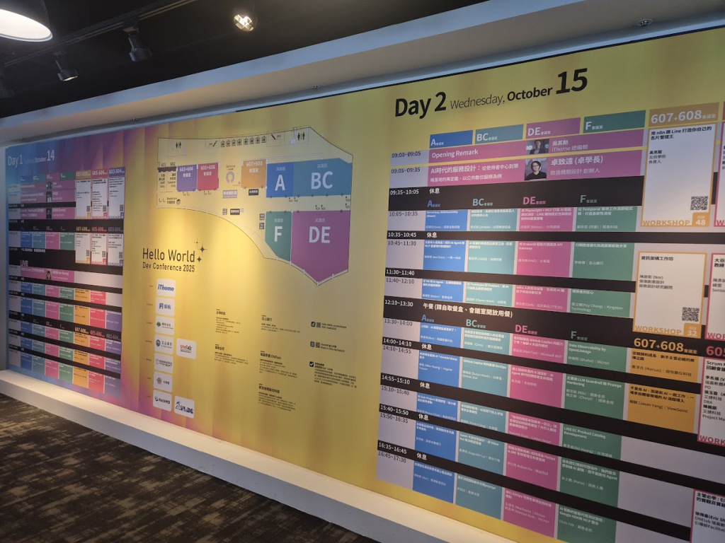
Greetings from Taipei!
I just spent two days at the Hello World Dev Conference 2025 in Taipei, and beneath the hype around cloud and AI, I observed a single, unifying theme: The industry is desperately building tools to cope with a complexity crisis of its own making.
The agenda was a catalog of modern systems engineering challenges. The most valuable sessions were the “踩雷經驗” (landmine-stepping experiences), which offered hard-won lessons from the front lines.
However, these talks raised a more fundamental question for me. We are getting exceptionally good at building tools to detect and recover from failure but are we getting any better at preventing it?
This post is not a simple translation of a Mandarin-language Taiwan conference. It is my analysis of the patterns I observed. I have grouped the key talks I attended into three areas:
- Cloud Native Infrastructure;
- Reshaping Product Management and Engineering Productivity with AI;
- Deep Dives into Advanced AI Engineering.
Feel free to choose to dive into the section that interests you most.

Session: Smart Pizza and Data Observability
This session was led by Shuhsi (林樹熙), a Data Engineering Manager at Micron. Micron needs no introduction, they are a massive player in the semiconductor industry, and their smart manufacturing facilities are a prime example of where data engineering is mission-critical.

Shuhsi’s talk, “Data Observability by OpenLineage,” started with a simple story he called the “Smart Pizza” anomaly.
He presented a scenario familiar to anyone in a data-intensive environment: A critical dashboard flatlines, and the next three hours are a chaotic hunt to find out why. In his “Smart Pizza” example, the culprit was a silent, upstream schema change.
His solution, OpenLineage, is a powerful framework for what we would call digital forensics. It is about building a perfect, queryable map of the crime scene after the crime has been committed. By creating a clear data lineage, it reduces the “Mean Time to Discovery” from hours of panic to minutes of analysis.
Let’s be clear: This is critical, valuable work. Like OpenTelemetry for applications, OpenLineage brings desperately needed order to the chaos of modern data pipelines.
It is a fundamentally reactive posture. It helps us find the bullet path through the body with incredible speed and precision. However, my main point is that our ultimate goal must be to predict the bullet trajectory before the trigger is pulled. Data lineage minimises downtime. My work with simulation, which will be explained in the next session, aims to prevent it entirely by modelling these complex systems to find the breaking points before they break.
Session: Automating a .NET Discrete Event Simulation on Kubernetes
My talk, “Simulation Lab on Kubernetes: Automating .NET Parameter Sweeps,” addressed the wall that every complex systems analysis eventually hits: Combinatorial explosion.
While the industry is focused on understanding past failures, my session is about building the Discrete Event Simulation (DES) engine that can calculate and prevent future ones.

西琳 – YouTube)
To make this concrete, I used the analogy of a restaurant owner asking, “Should I add another table or hire another waiter?” The only way to answer this rigorously is to simulate thousands of possible futures. The math becomes brutal, fast: testing 50 different configurations with 100 statistical runs each requires 5,000 independent simulations. This is not a task for a single machine; it requires a computational army.
My solution is to treat Kubernetes not as a service host, but as a temporary, on-demand supercomputer. The strategy I presented had three core pillars:
- Declarative Orchestration: The entire 5,000-run DES experiment is defined in a single, clean Argo Workflows manifest, transforming a potential scripting nightmare into a manageable, observable process.
- Radical Isolation: Each DES run is containerised in its own pod, creating a perfectly clean and reproducible experimental environment.
- Controlled Randomness: A robust seeding strategy is implemented to ensure that “random” events in our DES are statistically valid and comparable across the entire distributed system.

The final takeaway was a strategic re-framing of a tool many of us already use. Kubernetes is more than a platform for web apps. It can also be a general-purpose compute engine capable of solving massive scientific and financial modelling problems. It is time we started using it as such.

Session: AI for BI
Denny’s (監舜儀) session on “AI for BI” illustrated a classic pain point: The bottleneck between business users who need data and the IT teams who provide it. The proposed solution was a natural language interface, the FineChatBI, a tool designed to sit on top of existing BI platforms to make querying existing data easier.
His core insight was that the tool is the easy part. The real work is in building the “underground root system” which includes the immense challenge of defining metrics, managing permissions, and untangling data semantics. Without this foundation, any AI is doomed to fail.
This is a crucial step forward in making our organisations more data-driven. However, we must also be clear about what problem is being solved.
This is a system designed to provide perfect, instantaneous answers to the question, “What happened?”
My work, and the next category of even more complex AI, begins where this leaves off. It seeks to answer the far harder question: “What will happen if…?” Sharpening our view of the past is essential, but the ultimate strategic advantage lies in the ability to accurately simulate the future.
Session: The Impossibility of Modeling Human Productivity
The presented Jugg (劉兆恭) is a well-known agile coach and the organiser of Agile Tour Taiwan 2020. His talk, “An AI-Driven Journey of Agile Product Development – From Inspiration to Delivery,” was a masterclass in moving beyond vanity metrics to understand and truly improve engineering performance.
Jugg started with a graph that every engineering lead knows in their gut. As a company grows over time:
- Business grow (purple line, up);
- Software architecture and complexity grow (first blue line, up);
- The number of developers increases (second blue line, up);
- Expected R&D productivity should grow (green line, up);
- But paradoxically, the actual R&D productivity often stagnates or even declines (red line, down).

Jugg provided a perfect analogue for the work I do. He tackled the classic productivity paradox: Why does output stagnate even as teams grow? He correctly diagnosed the problem as a failure of measurement and proposed the SPACE framework as a more holistic model for this incredibly complex human system.
He was, in essence, trying to answer the same class of question I do: “If we change an input variable (team process), how can we predict the output (productivity)?”
This is where the analogy becomes a powerful contrast. Jugg’s world of human systems is filled with messy, unpredictable variables. His solutions are frameworks and dashboards. They are the best tools we have for a system that resists precise calculation.
This session reinforced my conviction that simulation is the most powerful tool we have for predicting performance in the systems we can actually control: Our code and our infrastructure. We do not have to settle for dashboards that show us the past because we can build models that calculate the future.

Session: Building a Map of “What Is” with GraphRAG
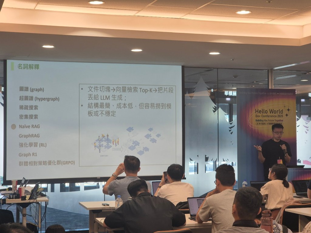
The most technically demanding session came from Nils (劉岦崱), a Senior Data Scientist at Cathay Financial Holdings. He presented GraphRAG, a significant evolution beyond the “Naive RAG” most of us use today.
He argued compellingly that simple vector search fails because it ignores relationships. By chunking documents, we destroy the contextual links between concepts. GraphRAG solves this by transforming unstructured data into a structured knowledge graph: a web of nodes (entities) and edges (their relationships).

In essence, GraphRAG is a sophisticated tool for building a static map of a known world. It answers the question, “How are all the pieces in our universe connected right now?” For AI customer service, this is a game-changer, as it provides a rich, interconnected context for every query.
This means our data now has an explicit, queryable structure. So, the LLM gets a much richer, more coherent picture of the situation, allowing it to maintain context over long conversations and answer complex, multi-faceted questions.
This session was a brilliant reminder that all advanced AI is built on a foundation of rigorous data modelling.
However, a map, no matter how detailed, is still just a snapshot. It shows us the layout of the city, but it cannot tell us how the traffic will flow at 5 PM.
This is the critical distinction. GraphRAG creates a model of a system at rest and DES creates a model of a system in motion. One shows us the relationships while the other lets us press watch how those relationships evolve and interact over time under stress. GraphRAG is the anatomy chart and simulation is the stress test.
Session: Securing the AI Magic Pocket with LLM Guardrails
Nils from Cathay Financial Holdings returned to the stage for Day 2, and this time he tackled one of the most pressing issues in enterprise AI: Security. His talk “Enterprise-Grade LLM Guardrails and Prompt Hardening” was a masterclass in defensive design for AI systems.
What made the session truly brilliant was his central analogy. As he put it, an LLM is a lot like Doraemon: a super-intelligent, incredibly powerful assistant with a “magic pocket” of capabilities. It can solve almost any problem you give it. But, just like in the cartoon, if you give it vague, malicious, or poorly thought-out instructions, it can cause absolute chaos. For a bank, preventing that chaos is non-negotiable.

There are two lines of defence: Guardrails and Prompt Hardening. The core of the strategy lies in understanding two distinct but complementary approaches:
- Guardrails (The Fortress): An external firewall of input filters and output validators;
- Prompt Hardening (The Armour): Internal defences built into the prompt to resist manipulation.
This is an essential framework for any enterprise deploying LLMs. It represents the state-of-the-art in building static defences.
While necessary, this defensive posture raises another important question for a developers: How does the fortress behave under a full-scale siege?
A static set of rules can defend against known attack patterns. But what about the unknown unknowns? What about the second-order effects? Specifically:
- Performance Under Attack: What is the latency cost of these five layers of validation when we are hit with 10,000 malicious requests per second? At what point does the defence itself become a denial-of-service vector?
- Emergent Failures: When the system is under load and memory is constrained, does one of these guardrails fail in an unexpected way that creates a new vulnerability?
These are not questions a security checklist can answer. They can only be answered by a dynamic stress test. The X-Teaming Nils mentioned is a step in this direction, but a full-scale DES is the ultimate laboratory.
Neil’s techniques are a static set of rules designed to prevent failure. Simulation is a dynamic engine designed to induce failure in a controlled environment to understand a system true breaking points. He is building the armour while my work with DES is in building the testing grounds to see where that armour will break.
Session: Driving Multi-Task AI with a Flowchart in a Single Prompt
The final and most thought-provoking session was delivered by 尹相志, who presented a brilliant hack: Embedding a Mermaid flowchart directly into a prompt to force an LLM to execute a deterministic, multi-step process.
He provided a new way beyond the chaos of autonomous agents and the rigidity of external orchestrators like LangGraph. By teaching the LLM to read a flowchart, he effectively turns it into a reliable state machine executor. It is a masterful piece of engineering that imposes order on a probabilistic system.
What he has created is the perfect blueprint. It is a model of a process as it should run in a world with no friction, no delays, and no resource contention.
And in that, he revealed the final, critical gap in our industry thinking.
A blueprint is not a stress test. A flowchart cannot answer the questions that actually determine the success or failure of a system at scale:
- What happens when 10,000 users try to execute this flowchart at once and they all hit the same database lock?
- What is the cascading delay if one step in the flowchart has a 5% chance of timing out?
- Where are the hidden queues and bottlenecks in this process?
His flowchart is the architect’s beautiful drawing of an airplane. A DES is the wind tunnel. It is the necessary, brutal encounter with reality that shows us where the blueprint will fail under stress.
The ability to define a process is the beginning. The ability to simulate that process under the chaotic conditions of the real world is the final, necessary step to building systems that don’t just look good on paper, but actually work.
Final Thoughts and Key Takeaways from Taipei
My two days at the Hello World Dev Conference were not a tour of technologies. In fact, they were a confirmation of a dangerous blind spot in our industry.
From what I observe, they build tools for digital forensics to map past failures. They sharpen their tools with AI to perfectly understand what just happened. They create knowledge graphs to model the systems at rest. They design perfect, deterministic blueprints for how AI processes should work.
These are all necessary and brilliant advancements in the art of mapmaking.
However, the critical, missing discipline is the one that asks not “What is the map?”, but “What will happen to the city during the hurricane?” The hard questions of latency under load, failures, and bottlenecks are not found on any of their map.
Our industry is full of brilliant mapmakers. The next frontier belongs to people who can model, simulate, and predict the behaviour of complex systems under stress, before the hurricane reaches.
That is why I am building SNA, my .NET-based Discrete Event Simulation engine.
I am leaving Taipei with a notebook full of ideas, a deeper understanding of the challenges and solutions being pioneered by my peers in the Mandarin-speaking tech community, and a renewed sense of excitement for the future we are all building.

