In cloud infrastructure, the ultimate challenge is building systems that are not just resilient, but also radically efficient. We cannot afford to provision hardware for peak loads 24/7 because it is simply a waste of money.
To achieve radical efficiency, AWS offers the T-series (like T3 and T4g). These instances allow us to pay for a baseline CPU level while retaining the ability to “burst” during high-traffic periods. This performance is governed by CPU Credits.
Modern T3 instances run on the AWS Nitro System, which offloads I/O tasks. This means nearly 100% of the credits we burn are spent on our actual SQL queries rather than background noise.
By default, Amazon RDS T3 instances are configured for “Unlimited Mode”. This prevents our database from slowing down when credits hit zero, but it comes with a cost: We will be billed for the Surplus Credits.
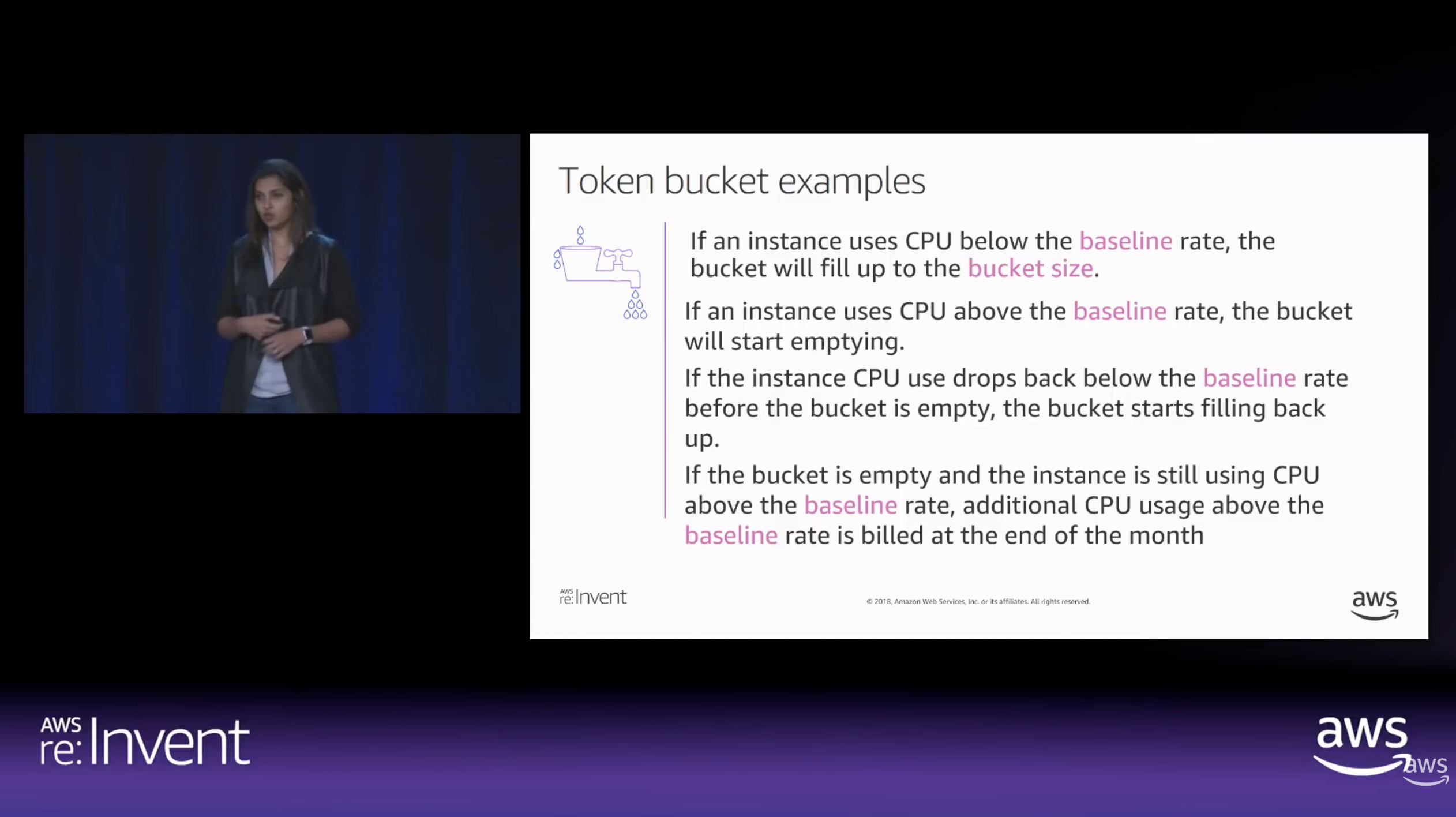
How CPU Credits are earned vs. spent over time. (Source: AWS re:Invent 2018)
The Experiment: Designing the Stress Test
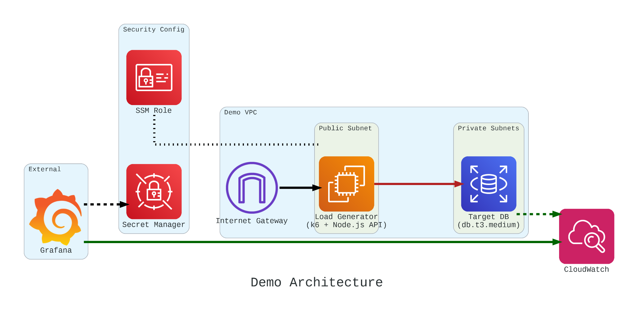
To truly understand how these credits behave under pressure, we built a controlled performance testing environment.
Our setup involved:
The Target: An Amazon RDS db.t3.medium instance.
The Generator: An EC2 instance running k6. We chose k6 because it allows us to write performance tests in JavaScript that are both developer-friendly and incredibly powerful.
The Workload: We simulated 200 concurrent users hitting an API that triggered heavy, CPU-bound SQL queries.
Simulation Fidelity with Micro-service
If we had k6 connect directly to PostgreSQL, it would not look like real production traffic. In order to make our stress test authentic, we introduce a simple NodeJS micro-service to act as the middleman.
This service does two critical things:
Implements a Connection Pool: Using the pg library Pool with a max: 20 setting, it mimics how a real-world app manages database resources;
Triggers the “Heavy Lifting”: The /heavy-query endpoint is designed to be purely CPU-bound. It forces the database to perform 1,000,000 calculations per request using nested generate_series.
In our k6 load test, we do not just flip a switch. We design a specific three-stage lifecycle for our RDS instance:
Ramp Up: We started with a gradual ramp-up from 0 to 50 users. This allows the connection pool to warm up and ensures we are not seeing performance spikes just from initial handshakes;
High-load Burn: We push the target to 200 concurrent users. These users will be hitting a /heavy-query endpoint that forces the database to calculate a million rows per second. This stage is designed to drain the CPUCreditBalance and prove that “efficiency” has its limits;
Ramp Down: Finally, we ramp back down to zero. This is the crucial moment in Grafana where we watch to see if the CPU credits begin to accumulate again or if the instance remains in a “debt” state.
import http from 'k6/http'; import { check, sleep } from 'k6';
export default function () { const res = http.get('http://localhost:3000/heavy-query'); check(res, { 'status was 200': (r) => r.status == 200 }); sleep(0.1); }
Monitoring with Grafana
If we are earning CPU credits slower than we are burning them, we are effectively walking toward a performance (or financial) cliff. To be truly resilient, we must monitor our CPUCreditBalance.
We use Grafana to transform raw CloudWatch signals into a peaceful dashboard. While “Unlimited Mode” keeps the latency flat, Grafana reveals the truth: Our credit balance decreases rapidly when CPU utilisation goes up to 100%.
Grafana showing the inverse relationship between high CPU Utilisation and a dropping CPU Credit Balance.
Predicting the Future with Discrete Event Simulation
Physical load testing with k6 is essential, but it takes real-time to run and costs real money for instance uptime.
Simulate a 24-hour traffic spike in just a few seconds;
Mathematically prove whether a rds.t3.medium is more cost-effective for a specific workload;
Predict exactly when an instance will run out of credits before we ever deploy it.
Simulation results from the SNA.
Final Thoughts
Efficiency is not just about saving money. Instead, it is about understanding the mathematical limits of our architecture. By combining AWS burstable instances with deep observability and predictive discrete event simulation, we can build systems that are both lean and unbreakable.
For those interested in the math behind the simulation, check out the SNA Library on GitHub.
In the previous article, we have discussed about how we can build a custom monitoring pipeline that has Grafana running on Amazon ECS to receive metrics and logs, which are two of the observability pillars, sent from the Orchard Core on Amazon ECS. Today, we will proceed to talk about the third pillar of observability, traces.
Source Code
The CloudFormation templates and relevant C# source codes discussed in this article is available on GitHub as part of the Orchard Core Basics Companion (OCBC) Project:https://github.com/gcl-team/Experiment.OrchardCore.Main.
Lisa Jung, senior developer advocate at Grafana, talks about the three pillars in observability (Image Credit: Grafana Labs)
We choose Tempo because it is fully compatible with OpenTelemetry, the open standard for collecting distributed traces, which ensures flexibility and vendor neutrality. In addition, Tempo seamlessly integrates with Grafana, allowing us to visualise traces alongside metrics and logs in a single dashboard.
Finally, being a Grafana Labs project means Tempo has strong community backing and continuous development.
About OpenTelemetry
With a solid understanding of why Tempo is our tracing backend of choice, let’s now dive deeper into OpenTelemetry, the open-source framework we use to instrument our Orchard Core app and generate the trace data Tempo collects.
OpenTelemetry is a Cloud Native Computing Foundation (CNCF) project and a vendor-neutral, open standard for collecting traces, metrics, and logs from our apps. This makes it an ideal choice for building a flexible observability pipeline.
OpenTelemetry provides SDKs for instrumenting apps across many programming languages, including C# via the .NET SDK, which we use for Orchard Core.
OpenTelemetry uses the standard OTLP (OpenTelemetry Protocol) to send telemetry data to any compatible backend, such as Tempo, allowing seamless integration and interoperability.
The http_listen_port allows us to set the HTTP port (3200) for Tempo internal web server. This port is used for health checks and Prometheus metrics.
After that, we configure where Tempo listens for incoming trace data. In the configuration above, we enabled OTLP receivers via both gRPC and HTTP, the two protocols that OpenTelemetry SDKs and agents use to send data to Tempo. Here, the ports 4317 (gRPC) and 4318 (HTTP) are standard for OTLP.
Last but not least, in the configuration, as demonstration purpose, we use the simplest one, local storage, to write trace data to the EC2 instance disk under /tmp/tempo/traces. This is fine for testing or small setups, but for production we will likely want to use services like Amazon S3.
In addition, since we are using local storage on EC2, we can easily SSH into the EC2 instance and directly inspect whether traces are being written. This is incredibly helpful during debugging. What we need to do is to run the following command to see whether files are being generated when our Orchard Core app emits traces.
ls -R /tmp/tempo/traces
The configuration above is intentionally minimal. As our setup grows, we can explore advanced options like remote storage, multi-tenancy, or even scaling with Tempo components.
Each flushed trace block (folder with UUID) contains a data.parquet file, which holds the actual trace data.
Finally, in order to enable Tempo to start on boot, we create a systemd unit file that allows Tempo to start on boot and automatically restart if it crashes.
cat <<EOF > /etc/systemd/system/tempo.service [Unit] Description=Grafana Tempo service After=network.target
systemctl daemon-reexec systemctl daemon-reload systemctl enable --now tempo
This systemd service ensures that Tempo runs in the background and automatically starts up after a reboot or a crash. This setup is crucial for a resilient observability pipeline.
Did You Know: When we SSH into an EC2 instance running Amazon Linux 2023, we will be greeted by a cockatiel in ASCII art! (Image Credit: OMG! Linux)
Understanding OTLP Transport Protocols
In the previous section, we configured Tempo to receive OTLP data over both gRPC and HTTP. These two transport protocols are supported by the OTLP, and each comes with its own strengths and trade-offs. Let’s break them down.
Ivy Zhuang from Google gave a presentation on gRPC and Protobuf at gRPConf 2024. (Image Credit: gRPC YouTube)
Tempo has native support for gRPC, and many OpenTelemetry SDKs default to using it. gRPC is a modern, high-performance transport protocol built on top of HTTP/2. It is the preferred option when performanceis critical. gRPC also supports streaming, which makes it ideal for high-throughput scenarios where telemetry data is sent continuously.
However, gRPC is not natively supported in browsers, so it is not ideal for frontend or web-based telemetry collection unless a proxy or gateway is used. In such scenarios, we will normally choose HTTP which is browser-friendly. HTTP is a more traditional request/response protocol that works well in restricted environments.
Since we are collecting telemetry from server-side like Orchard Core running on ECS, gRPC is typically the better choice due to its performance benefits and native support in Tempo.
Please take note that since gRPC requires HTTP/2, which some environments, for example, IoT devices and embedding systems, might not have mature gRPC client support, OTLP over HTTP is often preferred in simpler or constrained systems.
gRPC allows multiplexing over a single connection using HTTP/2. Hence, in gRPC, all telemetry signals, i.e. logs, metrics, and traces, can be sent concurrently over one connection. However, with HTTP, each telemetry signal needs a separate POST request to its own endpoint as listed below to enforce clean schema boundaries, simplify implementation, and stay aligned with HTTP semantics.
Logs:/v1/logs;
Metrics:/v1/metrics;
Traces:/v1/traces.
In HTTP, since each signal has its own POST endpoint with its own protobuf schema in the body, there is no need for the receiver to guess what is in the body.
AWS Distro for Open Telemetry (ADOT)
Now that we have Tempo running on EC2 and understand the OTLP protocols it supports, the next step is to instrument our Orchard Core to generate and send trace data.
The following code snippet shows what a typical direct integration with Tempo might look like in an Orchard Core.
This approach works well for simple use cases during development stage, but it comes with trade-offs that are worth considering. Firstly, we couple our app directly to the observability backend, reducing flexibility. Secondly, central management becomes harder when we scale to many services or environments.
ADOT is a secure, AWS-supported distribution of the OpenTelemetry project that simplifies collecting and exporting telemetry data from apps running on AWS services, for example our Orchard Core on ECS now. ADOT decouples our apps from the observability backend, provides centralised configuration, and handles telemetry collection more efficiently.
Sidecar Pattern
We can deploy the ADOT in several ways, such as running it on a dedicated node or ECS service to receive telemetry from multiple apps. We can also take the sidecar approach which cleanly separates concerns. Our Orchard Core app will focus on business logic, while a nearby ADOT sidecar handles telemetry collection and forwarding. This mirrors modern cloud-native patterns and gives us more flexibility down the road.
The following CloudFormation template shows how we deploy ADOT as a sidecar in ECS using CloudFormation. The collector config is stored in AWS Systems Manager Parameter Store under /myapp/otel-collector-config, and injected via the AOT_CONFIG_CONTENT environment variable. This keeps our infrastructure clean, decoupled, and secure.
Deploy an ADOT sidecar on ECS to collect observability data from Orchard Core.
There are several interesting and important details in the CloudFormation snippet above that are worth calling out. Let’s break them down one by one.
Firstly, we choose awsvpc as the NetworkMode of the ECS task. In awsvpc, each container in the ECS task, i.e. our Orchard Core container and the ADOT sidecar, receives its own ENI (Elastic Network Interface). This is great for network-level isolation. With this setup, we can reference the sidecar from our Orchard Core using its container name through ECS internal DNS, i.e. http://adot-collector:4317.
Secondly, we include a health check for the ADOT container. ECS will use this health check to restart the container if it becomes unhealthy, improving reliability without manual intervention. In November 2022, Paurush Garg from AWS added the healthcheck component with the new ADOT collector release, so we can simply specify that we will be using this healthcheck component in the configuration that we will discuss next.
Yes, the configuration! Instead of hardcoding the ADOT configuration into the task definition, we inject it securely at runtime using the AOT_CONFIG_CONTENT secret. This environment variable AOT_CONFIG_CONTENT is designed to enable us to configure the ADOT collector. It will override the config file used in the ADOT collector entrypoint command.
The SSM Parameter for the environment variable AOT_CONFIG_CONTENT.
Wrap-Up
By now, we have completed the journey of setting up Grafana Tempo on EC2, exploring how traces flow through OTLP protocols like gRPC and HTTP, and understanding why ADOT is often the better choice in production-grade observability pipelines.
With everything connected, our Orchard Core app is now able to send traces into Tempo reliably. This will give us end-to-end visibility with OpenTelemetry and AWS-native tooling.
I recently deployed an Orchard Core app on Amazon ECS and wanted to gain better visibility into its performance and health.
Instead of relying solely on basic Amazon CloudWatch metrics, I decided to build a custom monitoring pipeline that has Grafana running on Amazon EC2 receiving metrics and EMF (Embedded Metrics Format) logs sent from the Orchard Core on ECS via CloudFormation configuration.
In this post, I will walk through how I set this up from scratch, what challenges I faced, and how you can do the same.
Source Code
The CloudFormation templates and relevant C# source codes discussed in this article is available on GitHub as part of the Orchard Core Basics Companion (OCBC) Project:https://github.com/gcl-team/Experiment.OrchardCore.Main.
Why Grafana?
In the previous post where we setup the Orchard Core on ECS, we talked about how we can send metrics and logs to CloudWatch. While it is true that CloudWatch offers us out-of-the-box infrastructure metrics and AWS-native alarms and logs, the dashboards CloudWatch provides are limited and not as customisable. Managing observability with just CloudWatch gets tricky when our apps span multiple AWS regions, accounts, or other cloud environments.
The GrafanaLive event in Singapore in September 2023. (Event Page)
If we are looking for solution that is not tied to single vendor like AWS, Grafana can be one of the options. Grafana is an open-source visualisation platform that lets teams monitor real-time metrics from multiple sources, like CloudWatch, X-Ray, Prometheus and so on, all in unified dashboards. It is lightweight, extensible, and ideal for observability in cloud-native environments.
Is Grafana the only solution? Definitely not! However, personally I still prefer Grafana because it is open-source and free to start. In this blog post, we will also see how easy to host Grafana on EC2 and integrate it directly with CloudWatch with no extra agents needed.
Three Pillars of Observability
In observability, there are three pillars, i.e. logs, metrics, and traces.
Lisa Jung, senior developer advocate at Grafana, talks about the three pillars in observability (Image Credit: Grafana Labs)
Firstly, logs are text records that capture events happening in the system.
Secondly, metrics are numeric measurements tracked over time, such as HTTP status code counts, response times, or ECS CPU and memory utilisation rates.
Finally, traces show the form a strong observability foundation which can help us to identify issues faster, reduce downtime, and improve system reliability. This will ultimately support better user experience for our apps.
This is where we need a tool like Grafana because Grafana assists us to visualise, analyse, and alert based on our metrics, making observability practical and actionable.
Setup Grafana on EC2 with CloudFormation
It is straightforward to install Grafana on EC2.
Firstly, let’s define the security group that we will be use for the EC2.
ec2SecurityGroup:
  Type: AWS::EC2::SecurityGroup
  Properties:
    GroupDescription: Allow access to the EC2 instance hosting Grafana
    VpcId: {"Fn::ImportValue": !Sub "${CoreNetworkStackName}-${AWS::Region}-vpcId"}
    SecurityGroupIngress:
      - IpProtocol: tcp
        FromPort: 22
        ToPort: 22
        CidrIp: 0.0.0.0/0  # Caution: SSH open to public, restrict as needed
      - IpProtocol: tcp
        FromPort: 3000
        ToPort: 3000
        CidrIp: 0.0.0.0/0  # Caution: Grafana open to public, restrict as needed
      Tags:
        - Key: Stack
          Value: !Ref AWS::StackName
For demo purpose, please notice that both SSH (port 22) and Grafana (port 3000) are open to the world (0.0.0.0/0). It is important to protect the access to EC2 by adding a bastion host, VPN, or IP restriction later.
In addition, the SSH should only be opened temporarily. The SSH access is for when we need to log in to the EC2 instance and troubleshoot Grafana installation manually.
Now, we can proceed to setup EC2 with Grafana installed using the CloudFormation resource below.
In the CloudFormation template above, we are expecting our users to access the Grafana dashboard directly over the Internet. Hence, we put the EC2 in public subnet and assign an Elastic IP (EIP) to it, as demonstrated below, so that we can have a consistent public accessible static IP for our Grafana.
For production systems, placing instances in public subnets and exposing them with a public IP requires us to have strong security measures in place. Otherwise, it is recommended to place our Grafana EC2 instance in private subnets and accessed via Application Load Balancer (ALB) or NAT Gateway to reduce the attack surface.
Pump CloudWatch Metrics to Grafana
Grafana supports CloudWatch as a native data source.
With the appropriate AWS credentials and region, we can use Access Key ID and Secret Access Key to grant Grafana the access to CloudWatcch. The user that the credentials belong to must have the AmazonGrafanaCloudWatchAccess policy.
The user that Grafana uses to access CloudWatch must have the AmazonGrafanaCloudWatchAccess policy.
However, using AWS Access Key/Secret in Grafana data source connection details is less secure and not ideal for EC2 setups. In addition, AmazonGrafanaCloudWatchAccess is a managed policy optimised for running Grafana as a managed service within AWS. Thus, it is recommended to create our own custom policy so that we can limit the permissions to only what is needed, as demonstrated with the following CloudWatch template.
Again, using our custom policy provides better control and follows the best practices of least privilege.
With IAM role, we do not need to provide AWS Access Key/Secret in Grafana connection details for CloudWatch as a data source.
Visualising ECS Service Metrics
Now that Grafana is configured to pull data from CloudWatch, ECS metrics like CPUUtilization and MemoryUtilization, are available. We can proceed to create a dashboard and select the right namespace as well as the right metric name.
Setting up the diagram for memory utilisation of our Orchard Core app in our ECS cluster.
As shown in the following dashboard, we show memory and CPU utilisation rates because they help us ensure that our ECS services are performing within safe limits and not overusing or underutilizing resources. By monitoring the utilisation, we ensure our services are using just the right amount of resources.
Both ECS service metrics and container insights are displayed on Grafana dashboard.
Visualising ECS Container Insights Metrics
ECS Container Insights Metrics are deeper metrics like task counts, network I/O, storage I/O, and so on.
In the dashboard above, we can also see the number of Task Count. Task Count helps us make sure our services are running the right number of instances at all times.
Task Count by itself is not a cost metric, but if we consistently see high task counts with low CPU/memory usage, it indicates we can potentially consolidate workloads and reduce costs.
Instrumenting Orchard Core to Send Custom App Metrics
Now that we have seen how ECS metrics are visualised in Grafana, let’s move on to instrumenting our Orchard Core app to send custom app-level metrics. This will give us deeper visibility into what our app is really doing.
Metrics should be tied to business objectives. It’s crucial that the metrics you collect align with KPIs that can drive decision-making.
Metrics should be actionable. The collected data should help identify where to optimise, what to improve, and how to make decisions. For example, by tracking app-metrics such as response time and HTTP status codes, we gain insight into both performance and reliability of our Orchard Core. This allows us to catch slowdowns or failures early, improving user satisfaction.
SLA vs SLO vs SLI: Key Differences in Service Metrics (Image Credit: Atlassian)
By tracking response times and HTTP code counts at the endpoint level, we are measuring SLIs that are necessary to monitor if we are meeting our SLOs.
With clear SLOs and SLIs, we can then focus on what really matters from a performance and reliability perspective. For example, a common SLO could be “99.9% of requests to our Orchard Core API endpoints must be processed within 500ms.”
In terms of sending custom app-level metrics from our Orchard Core to CloudWatch and then to Grafana, there are many approaches depending on our use case. If we are looking for simplicity and speed, CloudWatch SDK and EMF are definitely the easiest and most straightforward methods we can use to get started with sending custom metrics from Orchard Core to CloudWatch, and then visualising them in Grafana.
var metricData = new MetricDatum
    {
        MetricName = metricName,
        Value = value,
        Unit = StandardUnit.Count,
        Dimensions = new List<Dimension>
        {
            new Dimension
            {
                Name = "Endpoint",
                Value = endpointPath
            }
        }
    };

var request = new PutMetricDataRequest
    {
        Namespace = "Experiment.OrchardCore.Main/Performance",
        MetricData = new List<MetricDatum> { metricData }
    };
In the code above, we see new concepts like Namespace, Metric, and Dimension. They are foundational in CloudWatch. We can think of them as ways to organize and label our data to make it easy to find, group, and analyse.
Namespace: A container or category for our metrics. It helps to group related metrics together;
Metric: A series of data points that we want to track. The thing we are measuring, in our example, it could be Http2xxCount and Http4xxCount;
Dimension:A key-value pair that adds context to a metric.
If we do not define the Namespace, Metric, and Dimensions carefully when we send data, Grafana later will not find them, or our charts on the dashboards will be very messy and hard to filter or analyse.
In addition, as shown in the code above, we are capturing the HTTP status code for our Orchard Core endpoints. We will then use PutMetricDataAsync to send the metric data PutMetricDataRequest asynchronously to CloudWatch.
The HTTP status codes of each of our Orchard Core endpoints are now captured on CloudWatch.
In Grafana, now when we want to configure a CloudWatch panel to show the HTTP status codes for each of the endpoint, the first thing we select is the Namespace, which is Experiment.OrchardCore.Main/Performance in our example. Namespace tells Grafana which group of metrics to query.
After picking the Namespace, Grafana lists the available Metrics inside that Namespace. We pick the Metrics we want to plot, such as Http2xxCount and Http4xxCount. Finally, since we are tracking metrics by endpoint, we set the Dimension to Endpoint and select the specific endpoint we are interested in, as shown in the following screenshot.
Using EMF to Send Metrics
While using the CloudWatch SDK works well for sending individual metrics, EMF (Embedded Metric Format) offers a more powerful and scalable way to log structured metrics directly from our app logs.
Before we can use EMF, we must first ensure that the Orchard Core application logs from our ECS tasks are correctly sent to CloudWatch Logs. This is done by configuring the LogConfiguration inside the ECS TaskDefinitionas we discussed last time.
Once the ECS task is sending logs to CloudWatch Logs, we can start embedding custom metrics into the logs using EMF.
Instead of pushing metrics directly using the CloudWatch SDK, we send structured JSON messages into the container logs. CloudWatch will then auto detects these EMF messages and converts them into CloudWatch Metrics.
The following shows what a simple EMF log message looks like.
When a log message reaches CloudWatch Logs, CloudWatch scans the text and looks for a valid _aws JSON object inside anywhere in the message. Thus, even if our log line has extra text before or after, as long as the EMF JSON is properly formatted, CloudWatch extracts it and publishes the metrics automatically.
An example of log with EMF JSON in it on CloudWatch.
After CloudWatch extracts the EMF block from our log message, it automatically turns it into a proper CloudWatch Metric. These metrics are then queryable just like any normal CloudWatch metric and thus available inside Grafana too, as shown in the screenshot below.
Metrics extracted from logs containing EMF JSON are automatically turned into metrics that can be visualised in Grafana just like any other metric.
As we can see, using EMF is easier as compared to going the CloudWatch SDK route because we do not need to change or add extra AWS infrastructure. With EMF, what our app does is just writing special JSON-format logs.
Then CloudWatch Metrics automatically extracts the metrics from those logs with EMF JSON. The entire process requires no new service, no special SDK code, and no CloudWatch PutMetric API calls.
Cost Optimisation with Logs vs Metrics
Logs are more expensive than metrics, especially when we are storing large amounts of data over time. This is also true when logs are stored at a higher retention rate and are more detailed, which means higher storage costs.
Metrics are cheaper to store because they are aggregated data points that do not require the same level of detail as logs.
CloudWatch treats each unique combination of dimensions as a separate metric, even if the metrics have the same metric name. However, compared to logs, metrics are still usually much cheaper at scale.
By embedding metrics into your log data via EMF, we are actually piggybacking metrics into logs, and letting CloudWatch extract metrics without duplicating effort. Thus, when using EMF, we will be paying for both, i.e.
Log ingestion and storage (for the raw logs);
The extracted custom metric (for the metric).
Hence, when we are leveraging EMF, we should consider expire logs faster if we only need the extracted metrics long-term.
Granularity and Sampling
Granularity refers to how frequent the metric data is collected. Fine granularity provides more detailed insights but can lead to increased data volume and costs.
Sampling is a technique to reduce the amount of data collected by capturing only a subset of data points (especially helpful in high-traffic systems). However, the challenge is ensuring that you maintain enough data to make informed decisions while keeping storage and processing costs manageable.
In our Orchard Core app above, currently the middleware that we implement will immediately PutMetricDataAsync to CloudWatch which will then not only slow down our API but it costs more because we need to pay when we send custom metrics to CloudWatch. Thus, we usually “buffer” the metrics first, and then batch-send periodically. This can be done with, for example, HostedService which is an ASP.NET Core background service, to flush metrics at interval.
using Amazon.CloudWatch; using Amazon.CloudWatch.Model; using Microsoft.Extensions.Hosting; using Microsoft.Extensions.Options; using System.Collections.Concurrent;
public class MetricsPublisher( IAmazonCloudWatch cloudWatch, IOptions<MetricsOptions> options, ILogger<MetricsPublisher> logger) : BackgroundService { private readonly ConcurrentBag<MetricDatum> _pendingMetrics = new();
public void TrackMetric(string metricName, double value, string endpointPath) { _pendingMetrics.Add(new MetricDatum { MetricName = metricName, Value = value, Unit = StandardUnit.Count, Dimensions = new List<Dimension> { new Dimension { Name = "Endpoint", Value = endpointPath } } }); }
In our Orchard Core API, each incoming HTTP request may run on a different thread. Hence, we need a thread-safe data structure like ConcurrentBag for storing the pending metrics.
Please take note that ConcurrentBag is designed to be an unordered collection. It does not maintain the order of insertion when items are taken from it. However, since the metrics we are sending, which is the counts of HTTP status codes, it does not matter in what order the requests were processed.
Finally, we can inject MetricsPublisher to our middleware EndpointStatisticsMiddleware so that it can auto track every API request.
Wrap-Up
In this post, we started by setting up Grafana on EC2, connected it to CloudWatch to visualise ECS metrics. After that, we explored two ways, i.e. CloudWatch SDK and EMF log, to send custom app-level metrics from our Orchard Core app:
Whether we are monitoring system health or reporting on business KPIs, Grafana with CloudWatch offers a powerful observability stack that is both flexible and cost-aware.
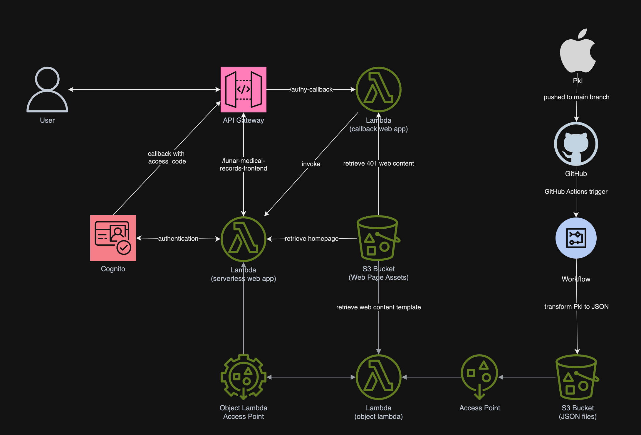
In the previous article, we talked about using the S3 Object Lambda to transform the medical records, which are stored in a JSON file, into a presentable web page. However, maintaining medical records in JSON files could be challenging. In this article, we will further investigate how we can generate those JSON files.
The part highlighted in red will be the focus of this article.
About Pkl
Pkl streamlines the creation of JSON scripts, enhancing maintainability and reducing verbosity through reuse, templating, and abstraction, all supported seamlessly right out of the box.
As we can expect from our medical records in JSON, the JSON files will grow larger over time. Hence it will be increasingly difficult to maintain. Pkl can help reduce the size and complexity of our JSON files by introducing abstractions for common elements and describing similar elements in terms of their differences.
Pkl comes with basic types, such as Numbers, Strings, Durations, etc. Having a notation for basic types, we can thus write typed objects. For example, the following module shows how we will define our medical records structure in Pkl.
module medicalVisitTemplate

class MedicalVisit {

    medicalCentreName: String

    centreType: "clinic"|"specialist"|"hospital"

    visitStartDate: Date

    visitEndDate: Date

    remark: String

    treatments: Listing<Treatment>

}

class Treatment {

    name: String

    type: "medicine"|"operation"|"scanning"

    amount: String

    startDate: Date

    endDate: Date

}

class Date {

    year: Int(isBetween(2000, 2100))

    month: Int(isBetween(1, 12))

    day: Int(isBetween(1, 31))
}

visits: Listing<MedicalVisit>
Listing is a collection in Pkl. It contains exclusively Elements, i.e., object members. In the code above, we define visits to be a collection of MedicalVisits. The MedicalVisit class contains information about the visit, for example type and name of the medical centres the patient visited, visiting period, remark, etc. The visiting period is then defined by Date class which stores year, month, and day.
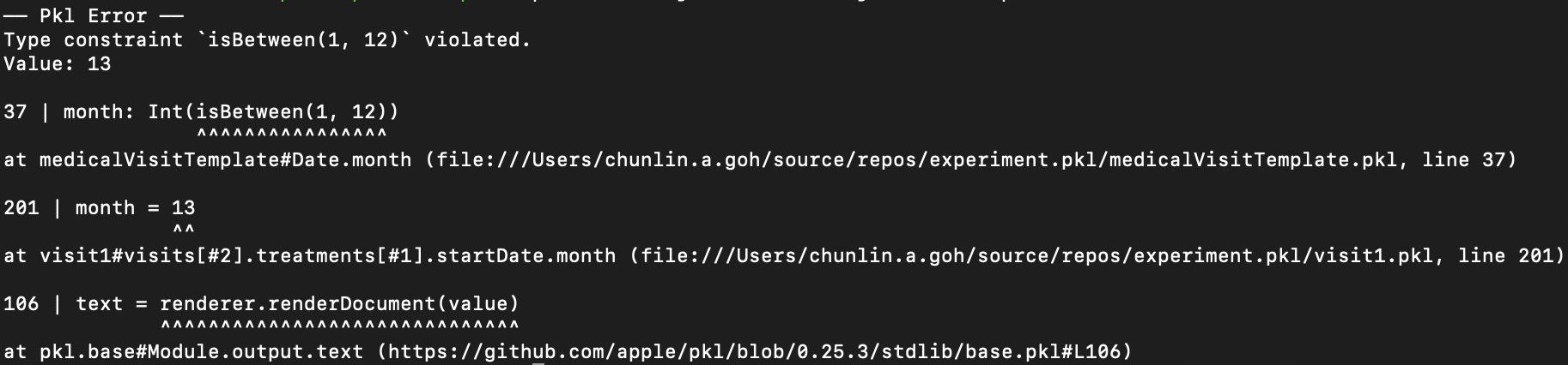
In the Date class, since the month can only be an integer from 1 to 12, so we can restrict it to an integer range by using Int and isBetween constraint. Later, as Pkl evaluates our configuration, if there is an invalid value, for example 13, provided to the month, there will be an error shown to us, as demonstrated below.
Pkl CLI will evaluate our configuration and show detected invalid values.
Generate JSON with Pkl
So now how do we generate JSON with the module above?
So, to generate the chunlin.json file that was shown in the previous blog post, we can amend the medicalVisitTemplate module above with another Pkl file called chunlin.pkl as shown below.
amends "medicalVisitTemplate.pkl"

visits = new Listing<MedicalVisit> {

    ...
    // Omitted for brevity

    new {

        medicalCentreName = "Tan Tock Seng Hospital"

        centreType = "hospital"

        visitStartDate {

            year = 2024

            month = 3

            day = 24

        }

        visitEndDate {

            year = 2024

            month = 4

            day = 19

        }

        remark = ""

        treatments = new Listing<Treatment> {

            ...
            // Omitted for brevity

            new {

                name = "Betamethasone (Valerate) 0.025% Cream 15g - Dermasone"

                type = "medicine"

                amount = "Applied after shower"

                startDate {

                    year = 2024

                    month = 3

                    day = 26

                }

                endDate {

                    year = 2024

                    month = 4

                    day = 19

                }

            }

            new {

                name = "Betamethasone (Valerate) 0.1% Cream 15g - Uniflex(TM)"

                type = "medicine"

                amount = "Applied after shower"

                startDate {

                    year = 2024

                    month = 3

                    day = 26

                }

                endDate {

                    year = 2024

                    month = 4

                    day = 19

                }

            }

        }

    }

}
Now if we execute the command below on Pkl CLI to evaluate the given modules and render the
With the command above, we can get the same output as we see in chunlin.json.
Maintain Pkl in GitHub
Static files like Pkl or JSON can be easily maintained in code repositories such as GitHub. Using GitHub for version control allows us to track changes to our PKL files over time. This makes it easy to revert to previous versions if something goes wrong, compare changes, and understand the evolution of our configuration files. Additionally, we can use GitHub Actions to automate various tasks related to our PKL files, enhancing efficiency and reliability in our workflow.
GitHub Actions is an automation tool that allows us to create workflows triggered by events within our repository. These workflows can automate tasks like testing, building, and deploying code, or even running scripts. By using GitHub Actions, we can streamline the development and transformation process of our Pkl files, ensure consistency, and improve efficiency.
Thus, our mission is now to configure GitHub Actions so that a JSON file can be produced from the Pkl file and sent to the Amazon S3 bucket that we setup in another article earlier.
Configure GitHub Actions Workflow
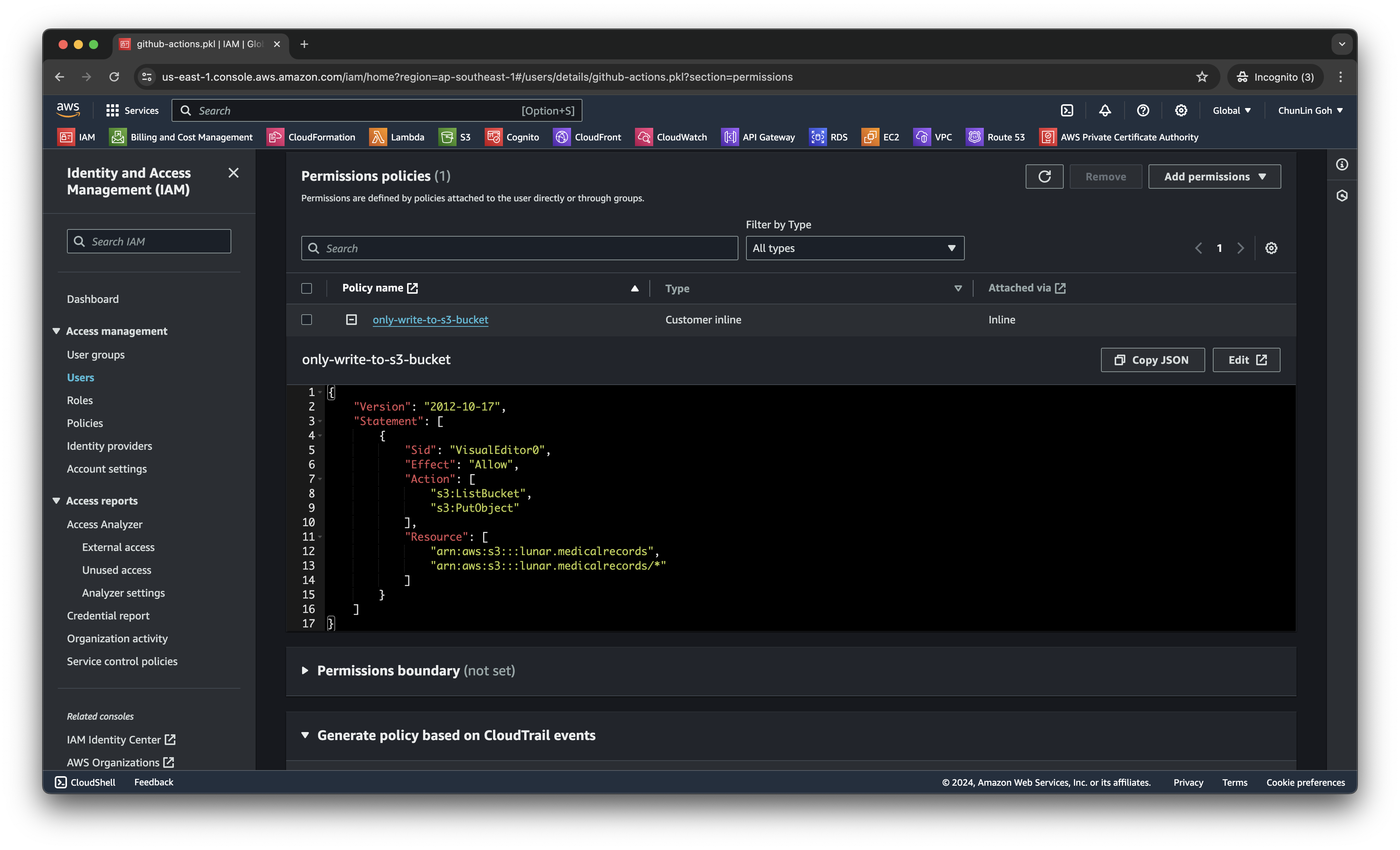
Firstly, we need to give permission to GitHub Actions to access our S3 bucket. To do so, we will create a new user in AWS Console with appropriate rights.
We only need two permissions, s3:ListBucket and s3:PutObject, to copy files from local to the S3 bucket.
After attaching the policy, we proceed to generate an access key for this newly created user.
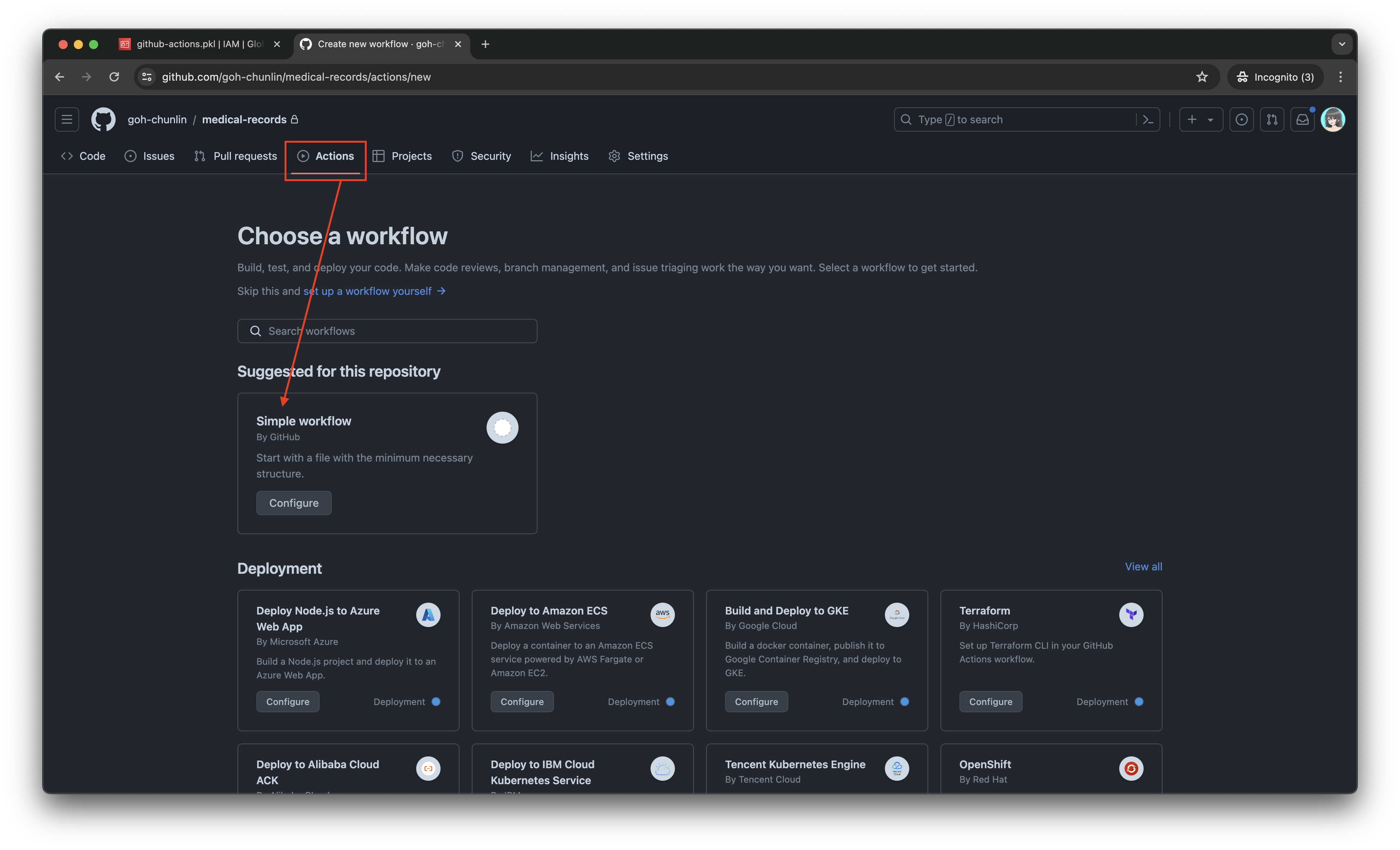
Secondly, we need to navigate to our repository and then click on the Actions tab to create a new simple workflow, as shown below.
- name: Install Linter run: go install github.com/Drafteame/pkl-linter@latest
- name: Run pkl-linter run: pkl-linter medical-records
The linter analyses our code and shows detected stylistic errors.
Next, we need to install the Pkl CLI to evaluate Pkl modules and write their output to a file. There are native executables available for us to use. As shown in the workflow above, the GitHub Actions runner is ubuntu-latest, which uses the Ubuntu 22.04 LTS image as of Jun 2024. It uses the amd64 architecture. Hence, we can download the Pkl Linux executable for amd64 architecture.
- name: Grant execute permission to Pkl CLI run: chmod +x pkl
- name: Get Pkl CLI version run: ./pkl --version
- name: Eval the Pkl files run: | cd medical-records files=$(find . -name "*.pkl") count=0 for file in $files; do output_filename="${file%.pkl}.json" ../pkl eval -f json -o ../output/$output_filename $file done cd ..
When my workflow is executed in June 2024, the version of the Pkl CLI is “Pkl 0.25.3 (Linux 5.15.0-1053-aws, native)”.
As shown in the last step above, it will loop through the JSON file in the medical-records folder and evaluate them one-by-one using the Pkl CLI. The JSON files generated will be stored in the output folder.
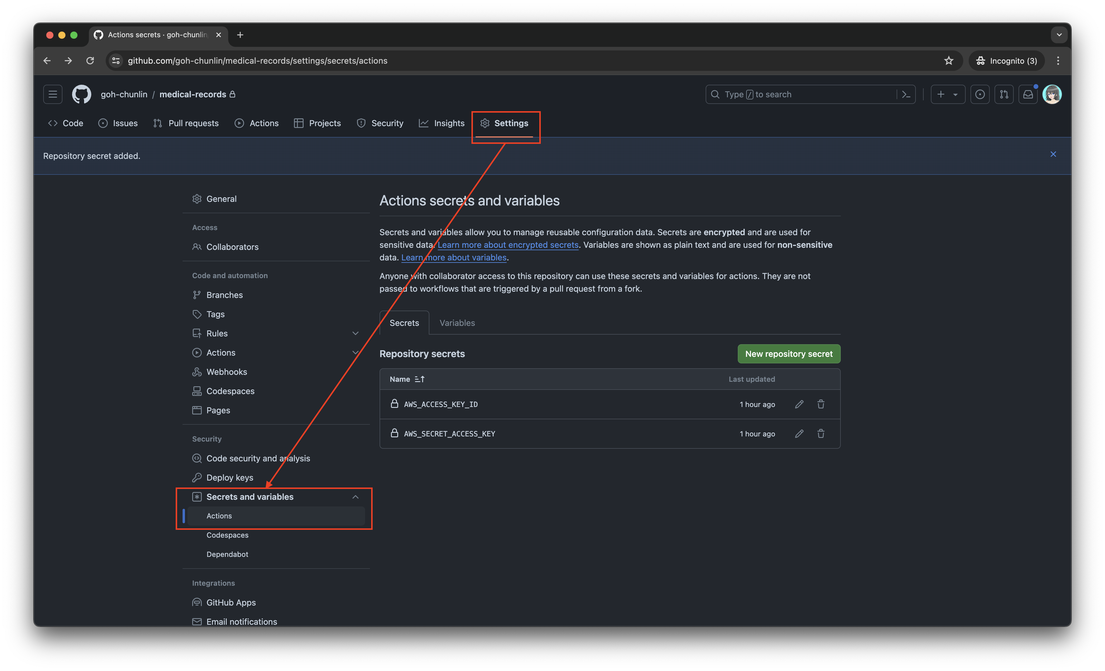
Eventually, what we need to do is to upload the file over to our AWS S3 bucket. However, before that, let’s make sure the AWS access key and secret access key we generated earlier are stored securely on GitHub Actions, a shown in the screenshot below.
The AWS access key and secret access key should be stored as GitHub Actions secrets.
Now, we can easily setup AWS CLI with the secrets above and use the s3 cp command to move the generated JSON files over to our S3 bucket. To do so, we only need to complete our workflow with the following.
In conclusion, utilising Pkl for generating and maintaining JSON files offers significant advantages in terms of reducing complexity and enhancing maintainability. By abstracting common elements and leveraging typed objects, Pkl simplifies the management of large and evolving datasets. The structured approach provided by Pkl not only minimises redundancy but also ensures that configurations remain consistent and error-free through its robust validation features.
Additionally, by using GitHub Actions, we can automate the process of evaluating Pkl files, generating the corresponding JSON files as output, and uploading these JSON files to our S3 bucket. This automation not only enhances efficiency but also ensures that changes are tracked and managed effectively.
In summary, we can conclude the infrastructure that we have gone through above and our previous article in the following diagram.